Introduction
HQS-UV-Vis provides UV/visible spectra with bands at the right position with a correct shape.
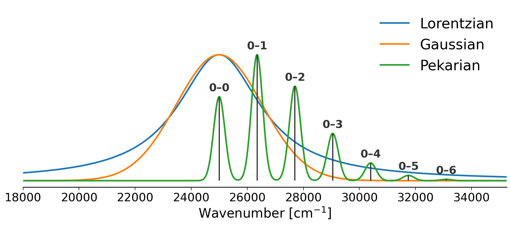
Electronic transitions are responsible for absorption and emission in the UV/Vis region. However, pure electronic transitions are an abstratction: in a more realistic picture electronic transitions are followed by changing of vibrational states, e.g. are vibronic = vibrational + electronic. Vibronic transitions define the fine structure of the electronic band, which is in non-trivial: in general it is asymmetric and can exhibit several maxima (so called vibronic progression). HQS-UV-Vis goes beyond pure electronic transition providing physically motivated and informative line shapes in the UV/Vis spectra.
What is HQS-UV-Vis?
HQS-UV-Vis is a toolkit for modeling ultraviolet and visible spectra in molecular systems using physically meaningful band shapes with a simple Python API. The package can compute spectra theoretically and fit theoretical models to experimental spectra. HQS-UV-Vis combines:
- Quantum-chemical calculations (DFTB+)
- Band/line shape models based on the Franck-Condon principle
- Advanced fitting algorithms for experimental electronic spectra
- Multi-state spectral analysis for complex electronic transitions
- Simple lineshape fitting (Gaussian, Lorentzian, Voigt)
- Flexible models: various line shapes for different bands
Key Features
Physical Models
- Franck-Condon Pekarian functions```
- Effective single-mode (ESM) approximations
- Linear coupling model (LCM) for Huang-Rhys factors
- Progressive broadening for inhomogeneous lineshapes
Theory Integration
- DFTB+ gradient and Hessian parsing
- Automatic normal mode analysis
- Multi-state vibronic spectra from multiple electronic states
- Theory-guided parameter initialization
- Automatic broadening parameter estimation
Visualization
- Spectrum comparison plots
- Vibronic progression decomposition
- Multi-component spectral fitting
Use Cases
HQS-UV-Vis is designed for:
- Experimental spectroscopists analyzing UV-Vis absorption or fluorescence
- Computational chemists visualizing quantum chemistry calculations
Getting Started
HQS UV Vis is included in the HQS Spectrum Tools module. To install it you need a running version of HQStage.
Once you have HQStage correctly configured you can install HQS Spectrum Tools using the command:
hqstage install hqs_spectrum_tools
Please note that HQS Spectrum Tools is currently only supported on Linux.
For using HQS UV Vis DFTB+ must be installed and available in your system PATH. You can obtain DFTB+ from:
- Using conda install "dftbplus=25.1=nompi_*"
- Official website: https://dftbplus.org/
- GitHub releases: https://github.com/dftbplus/dftbplus/releases
Verify your installation by running dftb+ in your terminal.
Slater-Koster Parameters
What are Slater-Koster files? Slater-Koster (SK) files contain the parametrized tight-binding integrals for element pairs (e.g., C-C, C-H, O-H). These are required for all DFTB+ calculations.
Download: SK parameter sets are available at: https://dftb.org/parameters/download.html
Recommendation: We recommend the 3ob-3-1 parameter set, which provides good accuracy for organic and biological molecules containing H, C, N, O, P, S, and halogens.
Continue to the Theory section to understand the theoretical foundations of UV/Vis spectral analysis.
License
HQS-UV-Vis is developed by HQS Quantum Simulations GmbH.
Copyright © 2026 HQS Quantum Simulations GmbH. All Rights Reserved.
Examples
This section documents two common workflows for hqs_uv_vis:
- Theoretical calculation of the guess spectrum
- Automatic fitting of theoretical model to the experiment
Both examples use the same input files (phthalimide.xyz and phthalimide_exp.npy) on publically accessable repository together with an examplary notebook.
Copyright © 2026 HQS Quantum Simulations GmbH. All Rights Reserved.
Theoretical calculation of the guess spectrum
This example shows how to generate theoretical initial parameter guesses using quantum-calculated transitions with DFTB+ as the backend. It loads the experimental spectrum to detect absorption bands for parameter initialization.
Note: The
sk_prefixparameter must point to the directory containing your locally downloaded Slater-Koster parameter files required by DFTB+. These are not included in the repository.
from pathlib import Path

from hqs_uv_vis.schema import default_angular_momentum, MoleculeStructure, WorkflowConfig
from hqs_uv_vis.api import AutoVibronicFitter
from hqs_uv_vis.preprocessing import SpectrumPreprocessor
from vibrofit.fitting.simple import detect_absorption_bands
from pydftb.io.parser import parse_xyzfile


def main() -> None:
    print("\nStarting Theoretical Guess Generation Pipeline...")
    DATA_DIR = Path(__file__).parent
    xyz_path = DATA_DIR / "phthalimide.xyz"
    molecule = MoleculeStructure(
            symbols=parse_xyzfile(xyz_path)["symbols"],
            coordinates=parse_xyzfile(xyz_path)["coordinates"],
    )
    print(f"✓ Loaded geometry containing {len(molecule.symbols)} atoms from {xyz_path.name}.")

    config = WorkflowConfig(
        band_types=["pekar", "pekar", "gaussian"],
        peak_prominence=0.05,
        dftb_command="dftb+",
        # Must point to the directory containing your downloaded Slater-Koster files.
        sk_prefix="/path/to/downloaded/slater-koster/3ob-3-1/", # Example path; update to your local location
        angular_momentum=default_angular_momentum(parse_xyzfile(xyz_path)["symbols"]),
        num_excitations=10,
        wavelength_range_nm=(200.0, 800.0),
        min_osc_strength=0.05,
    )

    exp_spectrum_path = DATA_DIR / "phthalimide_exp.npy"
    fitter = AutoVibronicFitter(config)

    print("\nPreprocessing Experimental Spectrum...")
    preprocessor = SpectrumPreprocessor(exp_spectrum_path)
    nu_exp, int_exp = preprocessor.get_conditioned_spectrum(smooth=False)

    print("\nDetecting Absorption Bands...")
    peak_nu_list = detect_absorption_bands(
        nu_exp, int_exp, prominence_thresh=config.peak_prominence
    )
    print(f"✓ Found {len(peak_nu_list)} peaks: {[round(p, 1) for p in peak_nu_list]} cm⁻¹")

    print("\nExecuting Quantum Calculations (or loading from cache)...")
    run_hash = fitter.cache.generate_hash(molecule, config)
    cached_data = fitter.cache.load_states(run_hash)

    if cached_data:
        print(f"✓ Cache HIT! Loaded quantum data. Hash: {run_hash}")
        data = cached_data
    else:
        print(f"✓ Cache MISS. Launching quantum orchestrator. Hash: {run_hash}")
        data = fitter.orchestrator.run_pipeline(molecule, debug=True)
        fitter.cache.save_states(run_hash, data)

    print("\nGenerating Theoretical Guesses...")
    p0, bounds, theory_results = fitter.generate_theoretical_guesses(
        data=data, peak_nu_list=peak_nu_list, nu_exp=nu_exp, debug=True
    )
Results
Running the example produces the following initial guess parameters:
| Band | Type | A | S | nu0 / cm^-1 | Omega / cm^-1 | sigma0 / cm^-1 | delta / cm^-1 | sigma / cm^-1 |
|---|---|---|---|---|---|---|---|---|
| 1 | Pekar | 1.000 | 1.936 | 46511.628 | 1303.390 | 459.250 | 130.339 | - |
| 2 | Pekar | 1.000 | 1.000 | 47511.628 | 1300.000 | 300.000 | 50.000 | - |
| 3 | Gaussian | 1.000 | - | 47511.628 | - | - | - | 300.000 |
Copyright © 2026 HQS Quantum Simulations GmbH. All Rights Reserved.
Automatic fitting of theoretical model to the experiment
This example shows how to run the full fitting workflow: execute the quantum calculations, fit the experimental spectrum, and save the results.
Note: The
sk_prefixparameter must point to the directory containing your locally downloaded Slater-Koster parameter files required by DFTB+. These are not included in the repository.
import numpy as np
from pathlib import Path

from hqs_uv_vis.schema import default_angular_momentum, MoleculeStructure, WorkflowConfig
from hqs_uv_vis.api import AutoVibronicFitter
from vibrofit.utils.printing import print_mixed_results, print_parameter_comparison
from vibrofit.plotting.summaries import plot_comprehensive_summary
from pydftb.io.parser import parse_xyzfile


def main() -> None:
    print("\nStarting Automated hqs_uv_vis Pipeline...")
    DATA_DIR = Path(__file__).parent
    xyz_path = DATA_DIR / "phthalimide.xyz"
    molecule = MoleculeStructure(
        symbols=parse_xyzfile(xyz_path)["symbols"],
        coordinates=parse_xyzfile(xyz_path)["coordinates"],
    )
    print(f"✓ Loaded geometry containing {len(molecule.symbols)} atoms from {xyz_path.name}.")

    config = WorkflowConfig(
        band_types=["pekar", "pekar", "gaussian"],
        peak_prominence=0.05,
        dftb_command="dftb+",
        # Must point to the directory containing your downloaded Slater-Koster files.
        sk_prefix="/path/to/downloaded/slater-koster/3ob-3-1/", # Example path; update to your local location
        angular_momentum=default_angular_momentum(parse_xyzfile(xyz_path)["symbols"]),
        num_excitations=10,
        wavelength_range_nm=(200.0, 800.0),
        min_osc_strength=0.05,
        run_bootstrap=False,
    )

    exp_spectrum_path = DATA_DIR / "phthalimide_exp.npy"
    fitter = AutoVibronicFitter(config)

    print("\nExecuting Quantum Calculations and Spectral Synthesis...")

    # Execution of the vibronic fitting spectrum workflow
    result = fitter.execute(molecule=molecule, exp_file=exp_spectrum_path, debug=True)

    if not config.run_bootstrap:
        print("✓ Skipping bootstrap error estimation for speed.")
    else:
        print("✓ Carrying out bootstrap error estimation.")
    print(f"✓ Optimization Converged! (R² = {result.r_squared:.5f})")

    print("\nFitting parameters for each band:")
    print_mixed_results(
        result.optimized_parameters, result.parameter_covariance, config.band_types
    )
    print(
        "Deviation between theoretic and fitted parameters for the "
        f"{len(result.theory_results['transitions'])} bright state(s)/band(s) found theoretically"
    )
    print_parameter_comparison(result.optimized_parameters, result.theory_results)

    output_dat = DATA_DIR / f"phthalimide_fitted_{result.strategy_used}.dat"
    np.savetxt(
        output_dat,
        np.column_stack(
            [
                result.final_spectrum["frequencies_cm1"],
                result.final_spectrum["intensities"],
                result.exp_spectrum["intensities"],
            ]
        ),
        header=f"Frequency (cm-1) | Fitted Intensity ({result.strategy_used}) | Exp. Intensity",
        fmt="%.6e",
    )

    plot_comprehensive_summary(
        result.exp_spectrum["frequencies_cm1"],
        result.exp_spectrum["intensities"],
        result.optimized_parameters,
        config.band_types,
        theory_results=result.theory_results,
        output_path=DATA_DIR / f"phthalimide_summary_{result.strategy_used}.png",
    )
    print(f"✓ Results saved to {DATA_DIR.name}/")
Result
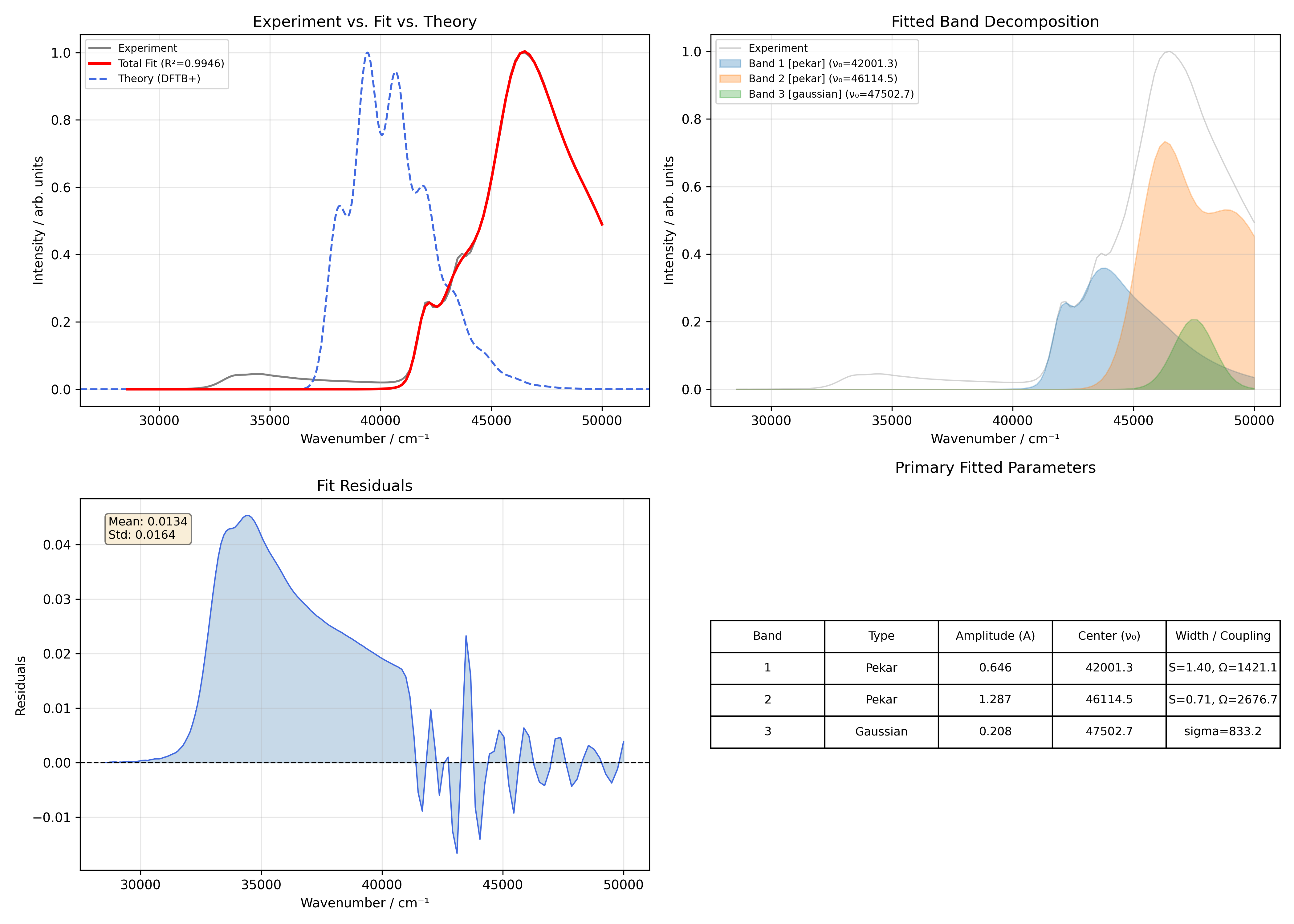
The resulting summary plot for the fitted phthalimide spectrum is shown below.
Copyright © 2026 HQS Quantum Simulations GmbH. All Rights Reserved.
Band shapes in UV/Visible spectra: Franck-Condon Principle
Let us consider an electronic transition from state to state . The intensity of the pure electronic transition is governed by the transition dipole moment :
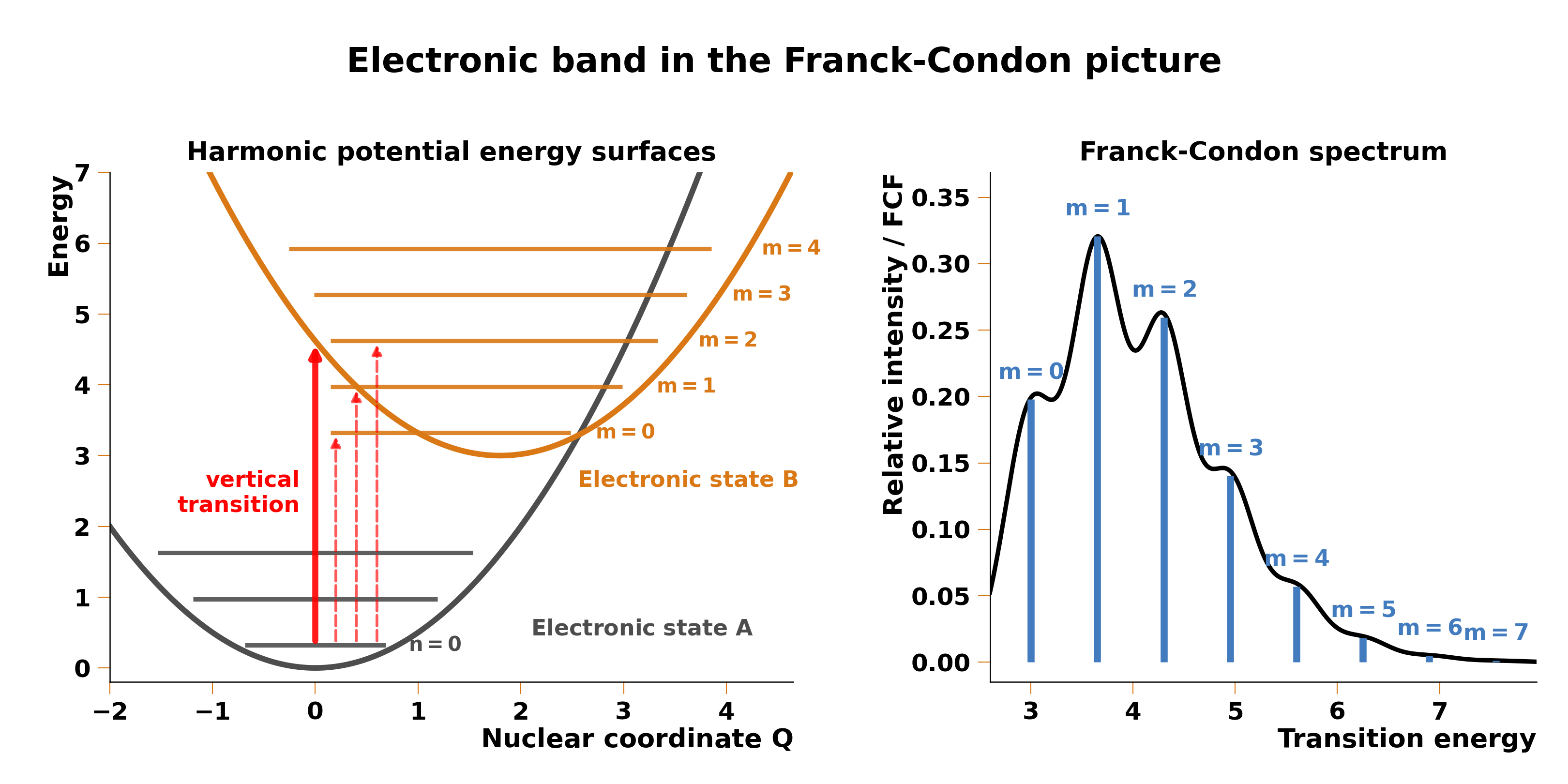
In reality, electronic transitions are accompanied by changes in the vibrational state of the molecule (vibronic transitions). Assuming only transitions from the ground vibrational state of electronic state , , (i.e., zero temperature) the intensity of vibronic transition from to is in the first approximation:
where is the electronic transition dipole moment, whereas is the Franck-Condon factor equal to the overlap of the vibrational wave functions in different electronic states. Thus an electronic band (for example in the UV/Visible absorption spectrum) consists of vibronic lines, which may or may not be resolved in the experiment. This shape is in general asymmetric unlike Lorentz and Gauss profiles.
References
- Franck, J. & Dymond, E. G. "Elementary processes of photochemical reactions," Trans. Faraday Soc. 21, 536-542 (1926). DOI: 10.1039/TF9262100536
- Condon, E. U. "A theory of intensity distribution in band systems," Phys. Rev. 28, 1182-1201 (1926). DOI: 10.1103/PhysRev.28.1182
Linear Coupling Model (LCM)
The Linear Coupling Model relates excited-state gradients to vibronic coupling. It assumes that vibrations in the electronically excited states have the same frequencies and normal modes and only differ by the origin shift (displacement).
Theory
Mathematically it means that the excited-state potential energy surface near the ground-state equilibrium geometry is:
where:
- : Excited-state energy at ground-state equilibrium geometry
- : Normal mode coordinates
- : Excited-state gradient at ground-state geometry
- : Ground-state Hessian
Huang-Rhys Factors from Gradients
For each normal mode we define the mode displacement: where is normal mode shift between ground and excited electronic states.
Within the linear coupling model (LC): whereas where:
- : Excited-state gradient projection onto mode
- : Ground-state mode frequency
- : Mode displacement (dimensionless)
- : Huang-Rhys factor (dimensionless)
Physical interpretation of : Huang-Rhys factor is equal to the molecular reorganization energy at vibronic transition expressed in the units of the vibration frequency:
In addition:
- : No vibronic coupling (purely electronic transition)
- : Weak coupling (0-0 transition dominates)
- : Moderate coupling (several vibronic bands visible)
- : Strong coupling (many vibronic bands, red-shifted maximum)
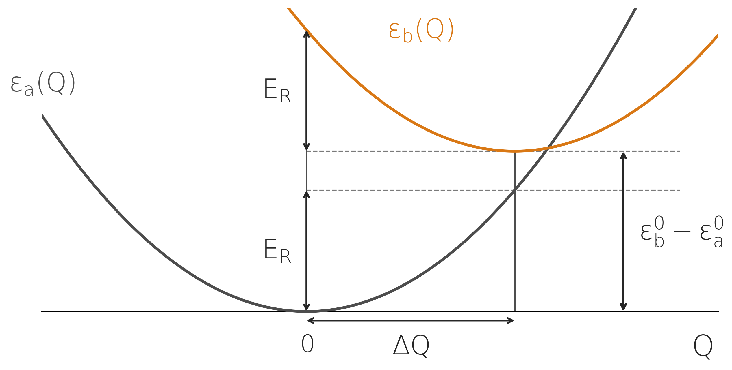
The vibronic profile of an electronic band in the linear coupling approximation follows a Poisson distribution for each mode with non-zero displacement: where is the vibrational state.
For several such active modes the spectrum is a convolution of Poisson distributions.
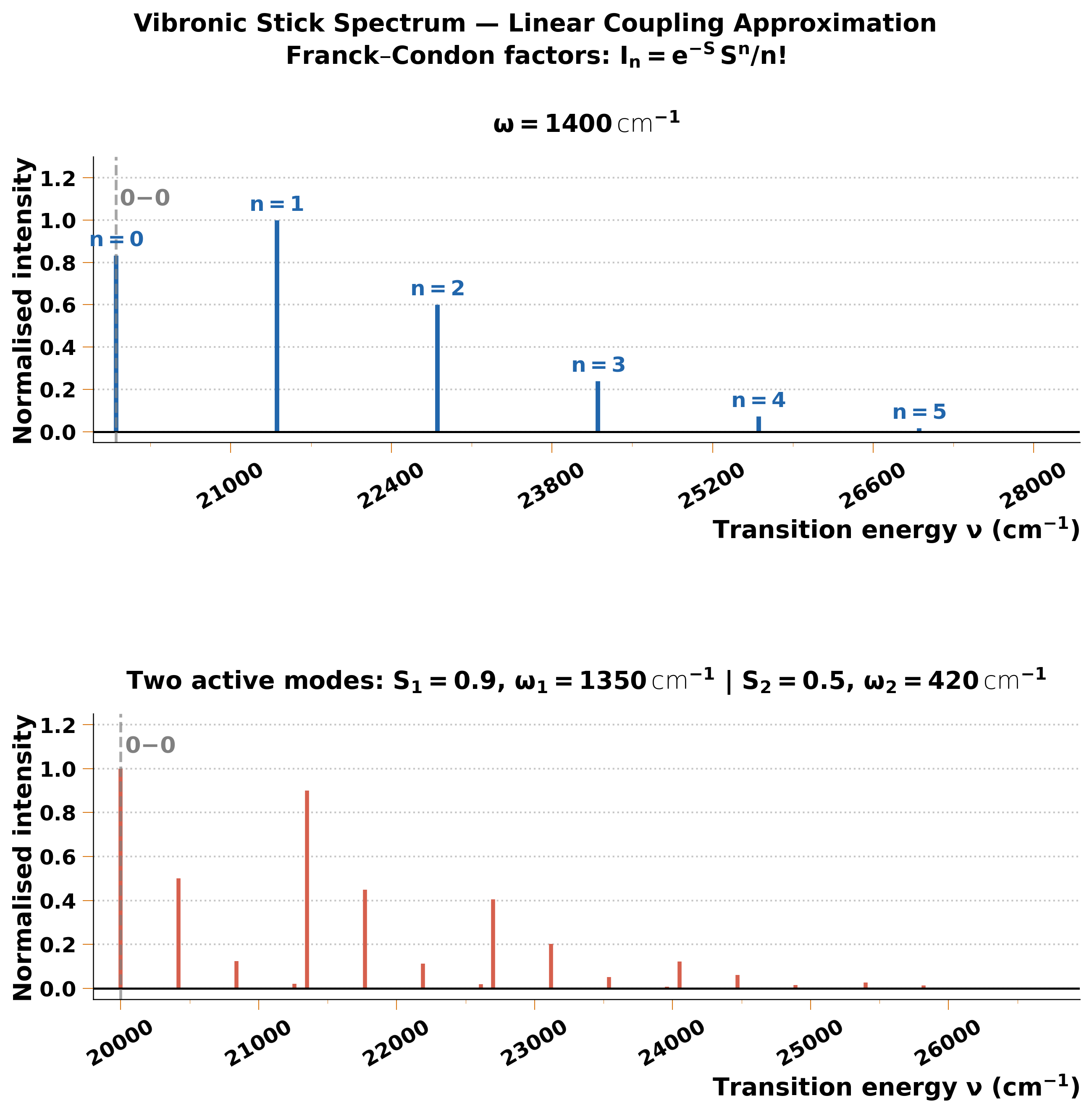
Computing vibronic profile within the LC model
- Ground state optimization
- Compute Hessian → frequencies and normal modes;
- Excited state gradient at ground-state geometry (vertical);
- Huang-Rhys factors: project Cartesian gradient onto normal modes; and calculate for each mode ;
- Generate spectrum as convolution of Poissonian distributions (Eq. 1).
Advantages
- Computationally efficient: Only need single-point gradient
- Physically motivated: Based on potential energy surfaces
- Mode-specific: Individual for each vibration
Limitations
- Harmonic approximation: Assumes quadratic potentials
- Linear coupling only: Neglects Duschinsky rotation and frequency changes
- Vertical approximation: Simplified geometry relaxation in the excited state
References
- Huang, K. & Rhys, A. "Theory of light absorption and non-radiative transitions in F-centres," Proc. R. Soc. Lond. A 204, 406-423 (1950). DOI: 10.1098/rspa.1950.0184
- Duschinsky, F. "Zur Deutung der Elektronenspektren mehratomiger Moleküle," Acta Physicochim. URSS 7, 551-566 (1937)
- Kupka, H. & Cribb, P. H. "Multidimensional Franck–Condon integrals and Duschinsky mixing effects," J. Chem. Phys. 85, 1303-1315 (1986). DOI: 10.1063/1.451216
Franck-Condon Pekarian Functions
The Pekarian function provides an analytical formulation of the Franck-Condon principle for vibronic spectra, using the Effective Single-Mode (ESM) approximation.
Key Concept: All vibrational modes are collapsed into a single effective mode with parameters (effective frequency) and (effective Huang-Rhys factor). This simplification matches the natural output of quantum chemistry ESM calculations.
Relation to multi-mode treatment: Both Pekarian (ESM) and multi-mode approaches implement Franck-Condon physics. Pekarian uses one effective mode (simpler, faster), while multi-mode treats each mode explicitly (more detailed, slower).
Definition
The absorption spectra using Pekarian models:
where:
- : Overall amplitude
- : Huang-Rhys factor
- : 0-0 transition frequency
- : Effective vibrational frequency
- : Progressive broadening
- : Lineshape function (Gaussian or Lorentzian)
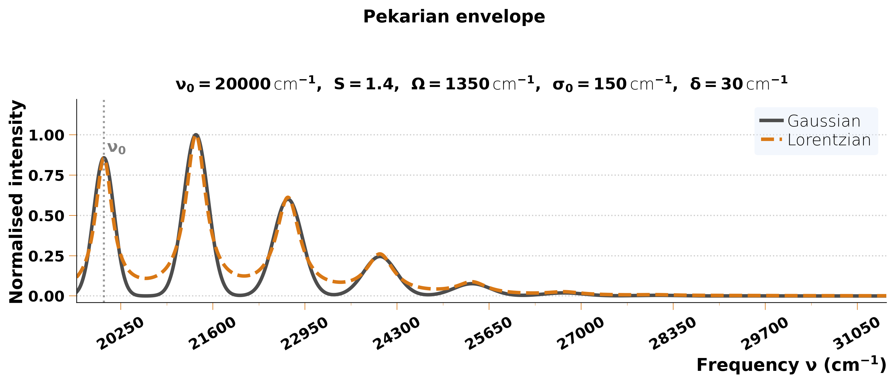
Physical Interpretation
The Pekarian function models:
- Poisson distribution: weights for quanta
- Vibronic progression: peaks at
- Progressive broadening: linewidth increases with
Parameters
| Parameter | Physical Meaning | Typical Range |
|---|---|---|
| Vibronic coupling strength | 0.1 - 2.0 | |
| Dominant vibration () | 800 - 2000 | |
| 0-0 linewidth () | 50 - 500 | |
| Width increment () | 10 - 200 |
Absorption vs. Fluorescence
Absorption (PFa):
- Progression to higher energy:
- Models ground → excited transitions
Fluorescence (PFf):
- Progression to lower energy:
- Models excited → ground emission
References
- Larina, N. & Khodorkovsky, V. "Pekarian Functions for Vibronic Spectra Analysis," New J. Chem. 49(10), 3937-3945 (2025). DOI: 10.1039/d4nj05537c
- Pekar, S. I., Zh. Eksp. Teor. Fiz. 20, 510 (1950)
Estimation of Pekarian Function Parameters for ESM Method
Overview
The Pekarian function for vibronic spectra in the ESM approximation requires five fundamental parameters:
with for progressive broadening.
| Parameter | Symbol | Physical Meaning | Source |
|---|---|---|---|
| 0-0 transition frequency | True spectroscopic 0-0 transition | From experiment | |
| Vertical excitation energy | QM approximation to | DFTB+/TD-DFT | |
| Effective Huang-Rhys factor | Total vibronic coupling strength | Linear coupling model | |
| Effective frequency | Dominant vibrational progression | Linear coupling model | |
| Initial linewidth | Width of 0-0 transition | Heuristic estimation | |
| Progressive broadening factor | Linewidth increase per quantum | Heuristic estimation |
Part I: Electronic and Vibronic Parameters from Quantum Chemistry
The first three parameters are obtained from quantum chemistry calculations combined with the LCM approximation.
I.A: Zero-Zero Transition Energy ()
Definition: The 0-0 transition frequency is the energy difference between the ground electronic state (v=0) and excited electronic state (v=0).
Calculation from quantum chemistry: The vertical excitation energy from DFTB+ serves as a computational approximation to . In practice, but may differ due to environmental effects (solvent, temperature, geometry relaxation).
I.B: Effective Huang-Rhys Factor ()
Definition: Total vibronic coupling strength summed over all active modes.
where mode-specific Huang-Rhys factors are:
with = excited state gradient projection onto normal mode , and = ground state frequency for mode .
Calculation steps:
- Ground state optimization → Hessian → normal modes , frequencies
- Excited state gradient at ground state geometry
- Project gradient:
- Calculate:
- Sum:
Physical meaning: Controls vibronic progression intensity distribution (Poisson):
Typical values: Rigid aromatics: 0.3-0.8; Flexible aromatics: 0.8-1.5; Charge-transfer states: 1.5-3.0
I.C: Effective Vibrational Frequency ()
Definition: Intensity-weighted mean frequency of all active modes.
where is the total reorganization energy.
Physical meaning: Determines spacing between vibronic peaks. Strongly coupled modes contribute more.
Typical values: Aromatic hydrocarbons: 1200-1600 cm⁻¹; Conjugated systems: 1400-1600 cm⁻¹
Summary: Parameters from Quantum Chemistry
| Parameter | Formula | Units | Source |
|---|---|---|---|
| From (TD-DFT/DFTB+) | cm⁻¹ or eV | approximates | |
| Dimensionless | LCM from gradients | ||
| cm⁻¹ | Weighted mean from LCM |
Workflow:
- Ground state: Optimize geometry, compute Hessian →
- Excited state: Compute gradient , energy (approximation to )
- LCM: Project gradient → , sum → , weighted average →
Part II: σ₀ Estimation (Initial Linewidth)
Physical meaning: The parameter represents the linewidth of the 0-0 transition, including inhomogeneous broadening, homogeneous broadening, and ESM approximation error.
Implemented Method: Dispersion
Calculates the weighted standard deviation of vibrational modes around the effective frequency. Directly measures how much the actual mode distribution deviates from the single effective mode approximation.
When to use: Default method. Provides physically meaningful measure of ESM quality. Gives reasonable values for typical organic molecules (50-300 cm⁻¹).
Typical Values and Guidelines
- Rigid systems (anthracene, rubrene): 50-150 cm⁻¹
- Flexible systems (polymers, solution): 200-400 cm⁻¹
- Disordered systems (amorphous films): 300-600 cm⁻¹
Sanity checks:
- Usually dispersion < cumulant
- Should be comparable to
- If , consider multi-mode method instead
Part III: δ Estimation (Progressive Broadening)
Physical meaning: The parameter represents progressive broadening with increasing vibrational quantum number: . Arises from anharmonicity, mode coupling, and lifetime effects.
Implemented Method: Linear scaling
Captures empirical observation that progressive broadening scales with ~10% of effective frequency, corresponding to typical anharmonicity in organic molecules.
Accuracy: ~15% average error for typical organic molecules. Range: 0.05-0.14 ×
Typical Values
For - cm⁻¹:
- typically: 50-200 cm⁻¹
- Corresponds to 5-15% of
- Gives - at
Empirical relationship: (typical)
Summary
| Parameter | Recommended Method | Typical Values | Key Formula |
|---|---|---|---|
| or | Experimental or (TD-DFT/DFTB+) | 15000-35000 cm⁻¹ | approximates |
| LCM from gradients | 0.3-3.0 | ||
| Weighted mean | 1200-1600 cm⁻¹ | ||
| Dispersion | 50-300 cm⁻¹ | ||
| Simple | 50-200 cm⁻¹ |
Complete workflow:
- Run quantum chemistry calculation (ground state Hessian + excited state gradient)
- Calculate (from ), , from LCM
- Auto-calculate (dispersion) and (simple)
- Validate against experimental data and refine by fitting if needed
Note: Parameters in this document are starting estimates from theory. Always validate and refine with experimental fitting when available. See Theory-Guided Fitting for full workflow integration.
Theory-Guided Fitting of UV/Visible Spectra
Overview
Theory-guided fitting uses quantum chemistry calculations as initial guesses for fitting experimental UV/visible spectra. This approach combines the strengths of both theoretical predictions (molecular properties like vibronic coupling and frequencies) and experimental measurements (accurate peak positions and intensities).
The method is particularly powerful for multi-component spectra with overlapping electronic transitions, where pure theory may miss environmental effects and manual fitting may miss physical constraints.
Complete Workflow
Step 1: Quantum Chemistry Calculations
- Ground state: optimize geometry, compute Hessian
- Excited states: compute gradients and energies for bright states
- Output: normal modes , gradients , excitation energies (approximation to )
Step 2: Linear Coupling Model Analysis
- Compute mode-specific Huang-Rhys factors from gradients (see Linear Coupling Model)
- Collapse to effective single mode: ,
- Estimate broadening parameters: , (see Estimation of Pekarian Parameters)
Step 3: Load Experimental Data
- Read experimental UV/Vis spectrum (wavenumber vs. intensity)
- Normalize intensity to [0,1] range
- Optionally smooth for peak detection
Step 4: Initial Parameter Guess
- Use theory for molecular properties: , , , (shapes and vibronic coupling)
- Use experiment for positions: from automatic peak detection
- Use experiment for amplitudes: from relative peak heights
- Set physical bounds (typically ±50% of theory values)
Step 5: Constrained Optimization
- Run minimization with boundaries with the L-BFGS-B algorithm (scipy.optimize.minimize)
- Enforce energy ordering constraint: (prevents band swapping)
- Monitor convergence (typically 10-50 iterations with good initial guess)
Step 6: Validation and Interpretation
- Check fit quality: , residuals - of max intensity
- Verify no systematic trends in residuals
- Compare fitted vs. theoretical parameters
Fitting Options
Function Types
- Lorentzian/Gaussian/Voigt: For broad, unresolved electronic bands
- Pekarian: For vibronically structured bands (see Pekarian Function)
- Mixed: Different function types for different peaks simultaneously
Constraint Options
- Energy ordering: Prevents band swapping during optimization ()
- Physical bounds: Limits parameters to reasonable ranges based on theory (±50% typical)
- Fixed parameters: Lock specific parameters if well-known from theory or prior fits
References
- Larina, N. & Khodorkovsky, V. "Pekarian Functions for Vibronic Spectra Analysis," New J. Chem. 49(10), 3937-3945 (2025). DOI: 10.1039/d4nj05537c
- Santoro, F., Lami, A., Improta, R., Bloino, J. & Barone, V. "Effective method for the computation of optical spectra of large molecules at finite temperature including the Duschinsky and Herzberg-Teller effect: The Qx band of porphyrin as a case study," J. Chem. Phys. 128, 224311 (2008). DOI: 10.1063/1.2929846