Automatic fitting of theoretical model to the experiment

This example shows how to run the full fitting workflow: execute the quantum calculations, fit the experimental spectrum, and save the results.

Note: The sk_prefix parameter must point to the directory containing your locally downloaded Slater-Koster parameter files required by DFTB+. These are not included in the repository.

import numpy as np
from pathlib import Path

from hqs_uv_vis.schema import default_angular_momentum, MoleculeStructure, WorkflowConfig
from hqs_uv_vis.api import AutoVibronicFitter
from vibrofit.utils.printing import print_mixed_results, print_parameter_comparison
from vibrofit.plotting.summaries import plot_comprehensive_summary
from pydftb.io.parser import parse_xyzfile


def main() -> None:
    print("\nStarting Automated hqs_uv_vis Pipeline...")
    DATA_DIR = Path(__file__).parent
    xyz_path = DATA_DIR / "phthalimide.xyz"
    molecule = MoleculeStructure(
        symbols=parse_xyzfile(xyz_path)["symbols"],
        coordinates=parse_xyzfile(xyz_path)["coordinates"],
    )
    print(f"✓ Loaded geometry containing {len(molecule.symbols)} atoms from {xyz_path.name}.")

    config = WorkflowConfig(
        band_types=["pekar", "pekar", "gaussian"],
        peak_prominence=0.05,
        dftb_command="dftb+",
        # Must point to the directory containing your downloaded Slater-Koster files.
        sk_prefix="/path/to/downloaded/slater-koster/3ob-3-1/", # Example path; update to your local location
        angular_momentum=default_angular_momentum(parse_xyzfile(xyz_path)["symbols"]),
        num_excitations=10,
        wavelength_range_nm=(200.0, 800.0),
        min_osc_strength=0.05,
        run_bootstrap=False,
    )

    exp_spectrum_path = DATA_DIR / "phthalimide_exp.npy"
    fitter = AutoVibronicFitter(config)

    print("\nExecuting Quantum Calculations and Spectral Synthesis...")

    # Execution of the vibronic fitting spectrum workflow
    result = fitter.execute(molecule=molecule, exp_file=exp_spectrum_path, debug=True)

    if not config.run_bootstrap:
        print("✓ Skipping bootstrap error estimation for speed.")
    else:
        print("✓ Carrying out bootstrap error estimation.")
    print(f"✓ Optimization Converged! (R² = {result.r_squared:.5f})")

    print("\nFitting parameters for each band:")
    print_mixed_results(
        result.optimized_parameters, result.parameter_covariance, config.band_types
    )
    print(
        "Deviation between theoretic and fitted parameters for the "
        f"{len(result.theory_results['transitions'])} bright state(s)/band(s) found theoretically"
    )
    print_parameter_comparison(result.optimized_parameters, result.theory_results)

    output_dat = DATA_DIR / f"phthalimide_fitted_{result.strategy_used}.dat"
    np.savetxt(
        output_dat,
        np.column_stack(
            [
                result.final_spectrum["frequencies_cm1"],
                result.final_spectrum["intensities"],
                result.exp_spectrum["intensities"],
            ]
        ),
        header=f"Frequency (cm-1) | Fitted Intensity ({result.strategy_used}) | Exp. Intensity",
        fmt="%.6e",
    )

    plot_comprehensive_summary(
        result.exp_spectrum["frequencies_cm1"],
        result.exp_spectrum["intensities"],
        result.optimized_parameters,
        config.band_types,
        theory_results=result.theory_results,
        output_path=DATA_DIR / f"phthalimide_summary_{result.strategy_used}.png",
    )
    print(f"✓ Results saved to {DATA_DIR.name}/")

Result

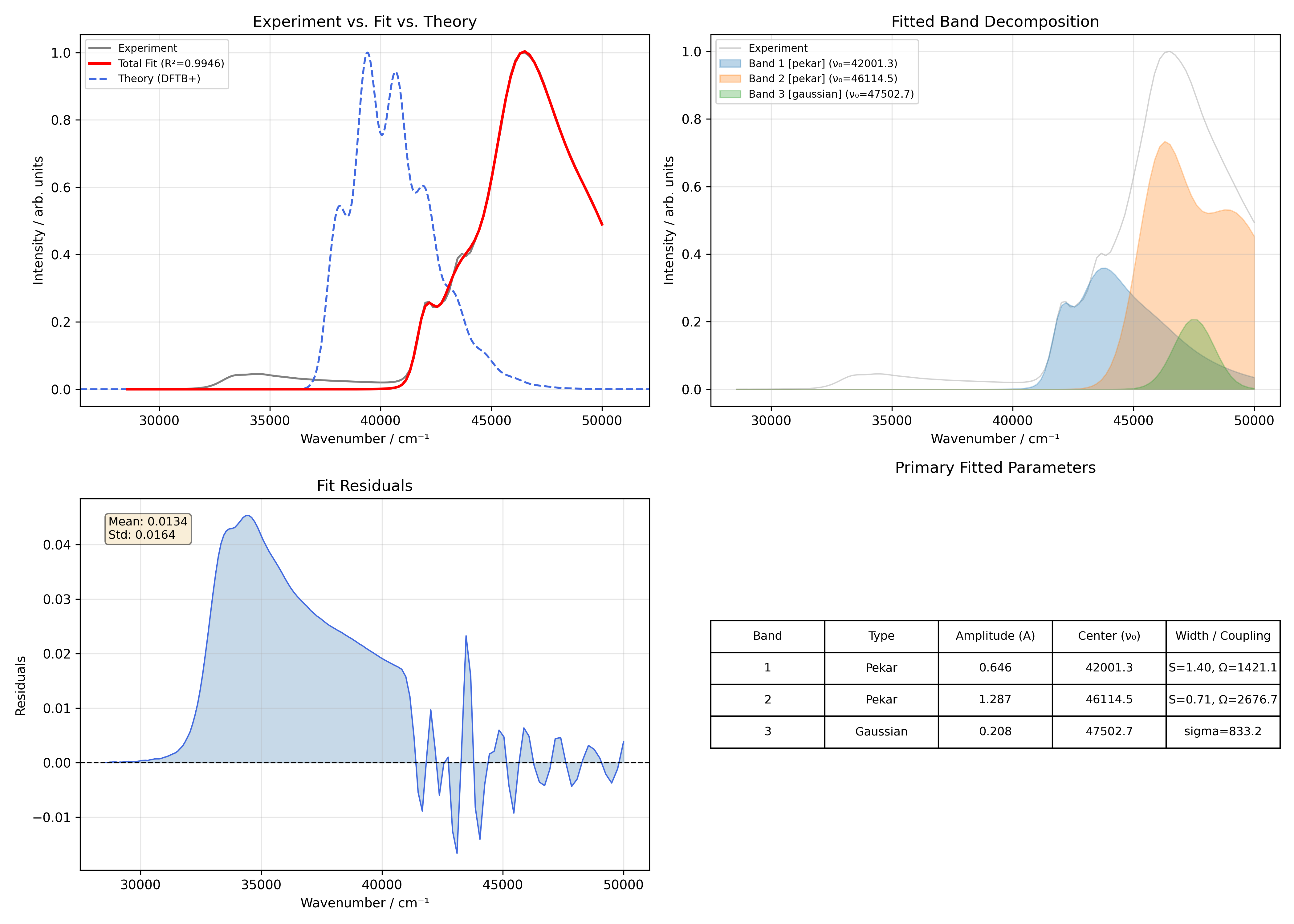
The resulting summary plot for the fitted phthalimide spectrum is shown below.

Summary plot for the fitted phthalimide spectrum

Keyboard shortcuts

HQS-UV-Vis Documentation

Automatic fitting of theoretical model to the experiment

Result