Introduction

The HQS Noise App offers a novel approach to mapping problems from diverse fields such as chemistry, materials science, and other quantum mechanical problems onto a quantum computer. What sets the HQS Noise App apart is its scalable approach to quantum simulation based on simulating time evolution.

This approach is designed for the simulation of mixed systems, e.g. spins coupled to fermions or bosons, which can be relevant for effects like light-matter interactions or microscopic vibrations in materials. It also provides novel capabilities for applications such as quantum machine learning. While the HQS Noise App is primarily tailored to NISQ devices, its relevance and significance extends to the era of fully error-corrected quantum computing. The Phase estimation algorithm, a key component for conducting quantum simulations on error-corrected quantum hardware, is based on the principle of time evolution. This principle is the cornerstone of the HQS Noise App, highlighting its continued importance in quantum computing.

Applications

The HQS Noise App can be used from two different perspectives:

1. To derive effective noisy algorithm models to gain insight into the effects of noise during circuit execution.
2. To use the noisy algorithm model to create optimized system-bath quantum circuits to simulate an open quantum system of interest on a noisy quantum computer.

The theoretical foundations of this software package have been published in two arxiv papers:

• noise mapping
• bath fitting.

For a detailed scientific discussion we refer the reader to the arxiv papers. This User Guide provides a concise summary of the fundamental physical concepts and an introduction to the Python interface of this software package.

Getting Started

First, HQStage has to be setup on the local machine (see the HQStage documentation for details).

The HQS Noise App can then be installed via the HQStage CLI tool with the following command

hqstage install hqs-noise-app

On the examples page, we show example analyses of several small-scale systems using the HQS Noise App. For more examples, see also our IPython notebook examples distributed along with the HQS Noise App.

Features

A changelog starting from version 0.5 can be found see here.

The Python API documentation can be found here.

Fundamental Physical Concepts

Noise Models

We consider physical noise, i.e. noise at the hardware level, caused by the coupling of qubits to some fluctuating environment, either during control operations or at all times. This is assumed to cause damping, dephasing, and/or depolarization of their quantum states. Our model of a noisy quantum computer is based on the addition of corresponding non-unitary (noise) operations after or before (ideal) unitary gate operations. This model is described in detail in the modeling section.

Noise Mapping

The first use of the HQS Noise App is to investigate how noise affects the gate-based quantum simulation of noiseless systems. Particularly, it solves the Lindblad open-system model that the noisy quantum hardware is effectively running. The foundations of this mapping (between physical and simulated noise) are discussed in the mapping section or in more detail in this arxiv paper. The mathematical derivation shown may be somewhat cumbersome in some places, but luckily the mathematics of connecting physical and effective noise for arbitrary quantum algorithms is done automatically by the HQS Noise App.

The System-Bath Approach

The second functionality of the HQS Noise App is to design system-bath quantum circuits to simulate an open quantum system of interest with the help of the physical noise on a quantum computer, thus turning parts of the noise on the device into a resource for computation by matching them to the dynamics of the studied bath. The basis of the system-bath approach is discussed in the system bath section of this user guide or in the arxiv paper.

Modeling Physical Noise

Background

We consider incoherent errors as the predominant noise mechanism in quantum simulation. These errors can arise from interactions between qubits and a fluctuating environment. This mechanism influences the time evolution of the qubits in a way that the errors do not add up coherently. Simple examples include superconducting qubits coupling to lossy two-level systems, ion trap devices with heated vibrational modes or unwanted control-pulse scattering, and spin qubits in the presence of fluctuating background magnetic-field. In recent decades, such noise mechanisms have been successfully described using the Lindblad master equation. The HQS Noise App applies this method to model the effect of noise in a digital quantum simulation.

Master Equation

Lindbladian

The noise mapping performed by the HQS Noise App is valid for noise mechanisms with short memory times, i.e. in the regime of Markovian dynamics. In particular, we apply master equations in the Lindbladian form:

\[ \dot{\rho} = \sum_{ij} M_{ij} \left( A_i \rho A^\dagger_j - \frac{1}{2} A^\dagger_j A_i \rho -\frac{1}{2} \rho A^\dagger_j A_i \right) \equiv L[\rho] , \]

where \(\rho\) is the density matrix of the qubits (spins). Operators \(A_i\) offer a basis for representing the noise operators, while matrix \(M\) provides (generalized) noise rates. There is a freedom in the definition of operators \(A_i\). Thus, only in combination with the matrix \(M\) (and particularly its non-diagonal entries) can we make judgements about the dominant noise processes and rates. In the following section we detail our choice of \(A_i\) operators so that the user can understand how their physical noise model can be represented by \(M\).

Noise Operators \(A\)

In our software, the \(A_i\) operators are chosen to be Pauli matrices, \(\sigma^x_n, \textrm{i}\sigma^y_n, \sigma^z_n\) (single-qubit noise on qubit \(n\)), and more generally Pauli products, \(\sigma^x_n\sigma^x_m,\sigma^x_n\textrm{i}\sigma^y_m,\sigma^x_n\sigma^z_m,\ldots\) (multi-qubit noise). An imaginary factor is added to Y operators ( \(\sigma^y_n\rightarrow \textrm{i}\sigma^y_n\) ) to avoid having imaginary numbers in the physical noise matrix \(M\). (The effective rate matrix, however, may end up having imaginary entries.)

Rate Matrix \(M\)

For clarity, we provide our definition of the spin-lowering and spin-raising operators:

\[ \sigma^-=\frac{1}{2}\left( \sigma^x + \textrm{i}\sigma^y \right) = \begin{pmatrix} 0 & 1 \\ 0 & 0 \end{pmatrix}, \\ \sigma^+=\frac{1}{2}\left( \sigma^x - \textrm{i}\sigma^y \right) = \begin{pmatrix} 0 & 0 \\ 1 & 0 \end{pmatrix} \]

The Lindblad equation for damping on qubit \(1\) has the form:

\[ \dot{\rho} = \gamma_{\textrm{damping}} \left( \sigma^-_1 \rho \sigma^+_1 - \frac{1}{2} \sigma^+_1 \sigma^-_1 \rho - \frac{1}{2} \rho \sigma^+_1 \sigma^-_1 \right) \]

\[ \dot{\rho} = \gamma_{\textrm{damping}} \left[ \frac{1}{4} \left( \sigma^x_1 + \textrm{i} \sigma^y_1 \right) \rho \left( \sigma^x_1 - \textrm{i} \sigma^y_1 \right) -\frac{1}{8} \left( \sigma^x_1 - \textrm{i} \sigma^y_1 \right) \left( \sigma^x_1 + \textrm{i} \sigma^y_1 \right) \rho -\frac{1}{8} \rho \left( \sigma^x_1 - \textrm{i} \sigma^y_1 \right) \left( \sigma^x_1 + \textrm{i} \sigma^y_1 \right) \right] . \]

Our noise matrix then has four non-zero values:

\[ M_{1X, 1X} = \frac{\gamma_\textrm{damping}}{4}, \\ M_{1X, 1 \textrm{i} Y} = \frac{\gamma_\textrm{damping}}{4}, \\ M_{1 \textrm{i} Y, 1X} = \frac{\gamma_\textrm{damping}}{4}, \\ M_{1 \textrm{i} Y, 1 \textrm{i} Y} = \frac{\gamma_\textrm{damping}}{4}. \]

Similarly, dephasing on qubit \(1\) corresponds to a noise matrix with a non-zero entry:

\[ M_{1Z, 1Z} = \gamma_\textrm{dephasing}. \]

Depolarization corresponds to identical noise in all directions with rates:

\[ M_{1X, 1X} = \frac{\gamma_\textrm{depolarising}}{4}, \\ M_{1Y, 1Y} = \frac{\gamma_\textrm{depolarising}}{4}, \\ M_{1Z, 1Z} = \frac{\gamma_\textrm{depolarising}}{4}. \]

This definition is based on the density matrix (here) approaching a diagonal matrix with rate \(\gamma_\textrm{depolarising}\).

Form of Noise Matrix \(M\) for the Physical Model

Since our physical noise acts individually on each qubit \(n\), our physical noise matrix is a sum over individual contributions \(m^n_{ij}\), where \(i,j\) can be \(nX,n\textrm{i}Y\) or \(nZ\). The matrix is real valued. In the case where noise acts on all qubits at all times, the total noise matrix has the form:

\[ M = m^0 \oplus m^1 \oplus m^2 \oplus \ldots , \]

whereas, if noise affects only qubits that are being operated on, we have:

\[ M = \bigoplus_{n\in \textrm{acted qubits}} m^n . \] It is important to note that this is the model for physical gates: the form of the effective noise can also include multi-qubit operators and imaginary (non-diagonal) rates, see sections mapping and examples.

Noisy Gates

Let us now introduce our model of gate-based quantum simulation with incoherent errors.

Superoperator Matrix Notation

For simplicity, we now use a notation where each noiseless gate (with a given unitary transformation \(U\)) is represented as a linear superoperator acting on the density matrix:

\[ U \rho U^{\dagger} = G \rho \\ U_2 U_1 \rho U_1^{\dagger} U_{2}^{\dagger} = G_2 G_1 \rho . \]

One can rewrite the right-hand side, such that the density "matrix" \(\rho\) has become a vector, and the unitary transformations \(G_i\) are matrices acting on it.

Model

In our modeling, we split each gate operation into the ideal unitary gate \(G\) and non-unitary noise \(N\). We then replace each gate in the gate decomposition with:

\[ G \rightarrow N G , \\ G_2 G_1 \rightarrow N_2 G_2 N_1 G_1 , \]

where the noise transformation is given by the Lindblad time evolution over some physical gate time \(\tau_i\),

\[ N_i \equiv e^{L\tau_i} , \]

where \(L\) is the Lindblad operator. Such a description can always be established when the physical gate times \(\tau_i\) are short in relation to the decoherence rates of this gate (\(\tau_i \gamma_i \ll 1\)), ensuring the noise to be small. A detailed justification of this model, including a proof that the separated noise term is a valid Lindblad operator (to the lowest order of the noise strength), can be found in our puplication on the subject. The question of how correct this description is of a specific hardware realization is then redirected to the question of the correct choice of noise matrix \(M\).

In the context of correctly describing the interplay of unitary gates and noise (see also the mapping section) the notion of so called small-angle gates is also important. In short, a small-angle gate is a unitary gate that is close to the identity gate compared to some other quantity of interest. The term is inspired by rotation gates (e.g. RotateX), which are close to the identity operation for small rotation angles. Small-angles are not an absolute quantity, but if we talk about unitary gates G together with noise contributions N with a small prefactor p, we would consider a unitary to be a small-angle gate if the deviation D of G from the identity is small enough compared to p that

\[ p GN = p NG + p [D,N] \approx p NG . \]

Foundations of noise mapping

In this section, we will go through the mathematical foundations of the noise mapping performed by the HQS Noise App. Physical noise on qubits is transformed into effective noise on spins in the quantum simulation. For a detailed discussion see the full paper on noise mapping.

Trotterization of the Time Evolution Operator

Decomposition Blocks

Digital quantum simulation is based on the trotterization of the time evolution operator, such that:

\[ e^{-\textrm{i} H t} = \left[ e^{-\textrm{i} H t/m} \right]^m \equiv \left[ e^{-\textrm{i} H \bar t} \right]^m \approx \left[ \Pi_{j} e^{-\textrm{i} H_j \bar t} \right]^m . \]

We consider a time-independent Hamiltonian \(H\) and time steps \(\bar t = t/m\). The total Hamiltonian \(H\) is divided into elements \(H_j\),

\[ H=\sum_j H_j . \]

Each \( H_j \) leads to a unitary transformation of the time evolution \(\exp\left(-\textrm{i} H_j\bar t \right)\), where the choice of a small value for \( \bar t \) makes this unitary transformation a "small-angle" transformation.

The goal of the division is to have a sequence of unitary transformations that can be efficiently implemented on hardware. In the HQS Noise App, such divisions are marked as circuit DecompositionBlocks. An approximation (error) occurs when individual unitaries do not commute.

Small- and Large-Angle Decompositions

Ideally, these unitaries can be implemented directly on hardware by single-qubit transitions or multi-qubit interactions, e.g., by control-field pulses. These operations then have a one-to-one correspondence with equivalent small-angle gates,

\[ e^{-\textrm{i} H_j \bar t} \rightarrow G_j . \]

As described in section modeling, in the presence of noise, each gate \(G_j\) is assigned a noise operator \(N_j\).

On the other hand, some unitaries may need to be decomposed into a series of elementary gates,

\[ e^{-\textrm{i} H_j \bar t} \rightarrow \Pi_l G^l_j . \]

Here, each gate \(G^l_j\) comes with noise \(N^l_j\). In practice, such decompositions often include "large-angle" gates, such as CNOT gates or \(\pi\) rotations.

Trotter Error

The error in the simplest, first-order, Trotter expansion is of size:

\[ \epsilon_\textrm{error} \propto \bar g^2 , \] where \(\bar g= g \bar t\), and \(g\) is some typical energy of non-commuting terms in the Hamiltonian. Note that the error goes to zero in the limit \(\bar t\rightarrow 0\).

Effective Noise in the Simulated System

Here, we detail how we map the physical noise of a quantum computer to effective noise in the simulated system. To do this, it is sufficient to analyze unitary gates and non-unitary noise operations within a single Trotter step. It also turns out that the analysis of noise rotations can be done on each decomposition block separately.

Noise Transformations

Let us first consider a decomposition of some small-angle unitary operation \(\exp\left(-\textrm{i} H_j\bar t \right)\) into two large-angle gates. The generalization to an arbitrary number of gates is straightforward.

Using the fact that gates \(G_i\) are unitary, and thereby invertible, we can write:

\[ N_2 G_2 N_1 G_1 \rho = N_2 G_2 N_1 G_2^{-1} G_2 G_1 \rho \equiv N_2 N_1' G_2 G_1 \rho \equiv N G \rho , \]

where \(G\) corresponds to a small-angle unitary operation (as it arises from a short time evolution),

\[ G = G_2 G_1 , \]

and the effective noise operator is:

\[ N = N_2 N_1' , \\ N'_1 = G_2 N_1 G_2^{-1} . \] We see that the first noise operator has been transformed by the (large-angle) unitary gate \(G_2\). Is is important to not that, since the operators \(G\) and \(N\) describe small-angle (or probability) processes, these operators will later define the effective Lindbladian of the simulated system.

More generally, for an arbitrary decomposition we can write:

\[ e^{-\textrm{i} H_j \bar t} \rightarrow \Pi_{l=\textrm{last}}^\textrm{first} N^l_j G^l_j = N_j G_j , \]

with:

\[ G_j \equiv \Pi_{l=\textrm{last}}^\textrm{first} G^l_j, \\ N_j \equiv \prod P_j \\ P_0 = N_j^\textrm{last} \\ P_1 = G_j^\textrm{last} N_j^\textrm{last-1} \left( G_j^\textrm{last}\right)^{-1} \\ P_2 = G_j^\textrm{last} G_j^\textrm{last-1} N_j^\textrm{last-2} \left( G_j^\textrm{last-1}\right)^{-1} \left( G_j^\textrm{last}\right)^{-1} \\ \ldots \]

It follows that the full time evolution operator can be written as:

\[ \Pi_j \exp\left( -\textrm{i} H_j\bar t \right) = \Pi_{j} N_j G_j . \]

Here, each operator \(G_j\) as well as \(N_j\) is a "small-angle" (or probability) transformation. Finally, within the assumption that rotations over small-angle transformations can be neglected, we obtain the expression for the full Trotter step:

\[ \Pi_{j} N_j G_j \approx \left(\Pi_j N_j \right) \left(\Pi_j G_j \right) = \left( \Pi_j N_j\right) G. \]

(Note that the SWAP algorithm for quantum simulation includes large-angle gates between decomposition blocks. However, the effect on the noise mapping, described above, is analogous to state swaps and can be accounted for by simple "reordering dictionaries" in decomposition block definitions.)

Lindbladian in the Simulated System

Noise mapping is most intuitively formulated in terms of unitary transformations of Lindbladian operators. When constructing the effective model Lindbladian, we include all consecutive noise operations \(N_j\), each of them being some multiplication of transformed Lindbladians \(N_j=\Pi_k\exp\left(L_j^k\tau_j^k\right)\) (see below), under one (exponentiated) Lindbladian,

\[ \Pi_j N_j = \Pi_{j} \Pi_{k} \exp\left(L_j^k\tau_j^k\right) \approx \exp\left(\sum_{jk} L_j^k\tau_j^k\right) \equiv \exp\left(L_\textrm{effective}\bar t\right), \]

where exponentiating the Lindbladian is shorthand notation for applying the full non-unitary time evolution. Here, each summed Lindbladian \(L_j^k\) has noise operators \(A_i\) that are conjugated by the unitary gate defined by its corresponding decomposition, \(O_j^k\equiv U_j^\textrm{last}U_j^\textrm{last-1}\ldots U_j^\textrm{k+1}\),

\[ A_{i} \rightarrow A_i^{jk} \equiv O_j^k A_i \left(O_j^k\right)^\dagger. \]

(For native gates there will be no transformation, so that for these \(A_i^{jk} = A_{i}\).) The final effective Lindbladian then takes the form:

\[ L_\textrm{effective}[\rho] \equiv \sum_{ii'jk} \frac{\tau_j^k}{\bar t} M^{jk}_{ii'}\left( S_1- \frac{1}{2}S_2\right). \]

with

\[ S_1 = A_i^{jk} \rho (A^{jk}_{i'})^\dagger \]

and the anti-commutator

\[ S_2 = \lbrace(A^{jk}_{i'})^\dagger A_i^{jk} , \rho \rbrace \]

Here, an important noise scaling factor \(\tau / \bar t\) appears. We can see that the effective noise decreases as the Trotter timestep \(\bar t\) increases. An example of this is given in the examples section.

Error in the Noise Mapping

The above approximations are analogous to neglecting the Trotter error. First, we made the approximation that noise transformations can be restricted to individual decomposition blocks. The error of this approximation is of size:

\[ \epsilon_\textrm{error} \propto \bar g \gamma \tau , \]

where \(\bar g= g \bar t\) and \(\gamma \tau\) are some typical Hamiltonian energy and noise probability of non-commuting elements between the superoperators of the noise and the unitary evolution. Importantly, the error goes to zero in the limit \(\bar t\rightarrow 0\).

Second, in the derivation of the Lindbladian, an error occurs when we combine consecutive noise terms (Lindbladians) under one exponent. This step has an error of size:

\[ \epsilon_\textrm{error} \propto (\gamma\tau)^2 \]

The validity of the noise mapping can be investigated numerically by comparing the solution for the original noisy circuit and for the effective Lindbladian, as shown in the examples section.

System-Bath Approach

The HQS Noise App generates quantum programs for quantum simulations of system-bath type problems. It is ideal for hardware with one or several good qubits, identified as the system qubits, which have weak noise compared to the other qubits, used as bath qubits. This version supports the simulation of spin-boson and spin-fermion systems. The boson or fermion baths are represented by bath spins.

The system-bath section is organised as follows:

1. System-Bath: an Overview
2. Using the HQS Noise App for System-Bath Approaches
3. System-Bath Functions
4. The Spin-Boson Model
5. Coarse Graining Details

We recommend reading through this section of the user documentation in the above order.

Quick Overview

Main idea: Utilizing Bath-Qubit Noise

In the HQS approach, noise originating in the bath qubits is effectively filtered and coupled to the system in a way that it appears to come from a bath with a continuous spectral function. This spectral function can be digitally tuned. We optimize the parameters of this system so that it reproduces the spectral function of a given system-bath problem. The optimization is performed using a finite number of bath-mode frequencies, system-bath couplings, and bath-mode broadenings. In the quantum simulation, the frequencies and couplings can be implemented digitally. Their magnitude is scaled so that the energy level broadenings due to the bath noise match to the fitting values. We also provide a SWAP algorithm specifically tailored for system-bath type problems, which takes into account that the bath is non-interacting.

In this version we provide functions to derive constraints for the broadening of the bath qubits from an available device. Providing these constraints to the optimization, the HQS Noise App will automatically optimize the utilization of the noisy qubits to improve the simulation results.

Validity

System-bath simulations are best implemented when:

• the system qubits have vanishing or weak noise.
• the effective noise of the bath qubits is predominantly damping and dephasing.
• the quantum computer has a two-dimensional architecture or all-system to all-bath connectivity.

However, these restrictions can be lifted with the cost of reduced simulation accuracy or by adding modifications to the system-bath model we simulate. For example, various types of noise mechanisms can be included to be a part of the simulation via changes in the form of the spin-boson Hamiltonian. Also, moderate system noise can be included as a constant background in the spectral functions, leading to an increased effective temperature.

Using the HQS Noise App

The objective is to start from a system-bath model (spin-boson or spin-fermion) that one wishes to simulate. This system-bath model is a mixed-system object (see also the struqture documentation) and can have either a dense spectrum of bath modes or a few broad bath modes. It is important the bath can be described by a spectral function according to normal Bloch-Redfield theory, as the bath will later be coarse-grained by the provided fitting tools. The output of the HQS Noise App will be a coarse-grained spin-boson system with optimized parameters. This system can then be turned into a mixed spin-spin system. The final total system is ideally small enough to be simulated on a quantum computer.

In this process, the fitting tool will also provide the best choice of Trotter time step when converting the spin-spin system into a quantum circuit that implements the time propagation under the spin-spin Hamiltonian. Choosing the right Trotter time step gives the best possible fit between the time evolution of the open system and the time propagation on the quantum computer under the influence of physical noise.

Coarse-Graining Mixed Hamiltonians

More detailed, the goal of using the tool is to convert either a spin-boson system (MixedLindbladOpenSystem) into a spin-spin system (MixedHamiltonian). The spin-boson system corresponds to a Hamiltonian of type:

\[ H_\textrm{input} = H_\textrm{system} + \frac{1}{2}\sum_{i} \sigma^i_x X_i + \sum_{m} \omega_{m} a^\dagger(\omega_m) a(\omega_m) \nobreakspace , \]

where the coupling between the system and the bath is described by spin-boson operators, where the spin parts are single-spin operators, and the bosonic part is a linear operator of the form:

\[ X_i = \sum_{m} g_{im} \left[a(\omega_m) + a^\dagger(\omega_m)\right] \nobreakspace . \]

The bosonic bath is non-interacting and has discretized frequencies \( \omega_m \) and widths \(d\omega_m\equiv \gamma_m\). The influence of such a bosonic bath on the system can be described by a spectral function. The widths are identified as boson-mode damping rates, corresponding to Lorentzian spectral peaks at their frequencies. All of the bosonic parts can also be given by a spectral function:

\[ S_{ij}(\omega) = 2\pi \sum_{m} g_{im}g_{jm} \delta(\omega-\omega_m + \textrm{i}\gamma_m) \nobreakspace , \]

added with the information of the interaction type, which, in this example, is \(\sigma_x \).

The final objective is to create a Hamiltonian of type MixedHamiltonian, with system spins and bath spins of the form:

\[ H_\textrm{output} = H_\textrm{system} + \sum_{i\in\textrm{system}}\sum_{j\in\textrm{bath}} \frac{g_{ij}}{2} \sigma_x^i\sigma_x^j + \sum_{j\in\textrm{bath}} \frac{\epsilon_j}{2} \sigma_z^j \nobreakspace . \]

The first part of the mixed system is the original spin-system. The second part is the effective spin-bath, which approximates the behaviour (spectral function) of the original bosonic bath. The broadening of the spin-bath modes is implemented by intrinsic noise of the qubits during the quantum simulation. This can be due to qubit damping and dephasing.

A more detailed technical description of the main functions used in the coarse-graining can be found in the simulation examples.

Creating Mixed Hamiltonians and Open Systems

The system-bath model is defined in the interface as a mixed system. The mixed system can have either two spin subsystems (a spin system and a spin bath), or one spin system and several bosonic subsystems. The bosonic subsystems are used to define the spin-boson problem. Note that only non-interacting baths are allowed, as explained in the section above. The corresponding system-bath couplings are limited to products of two Pauli operators.

In the following we create a spin-boson Hamiltonian with struqture_py. Struqture is a library that supports the building of spin objects, bosonic objects, fermionic objects and mixed system objects that contain arbitrarily many spin, fermionic and bosonic subsystems. The struqture documentation contains several examples of how to define different kinds of Hamiltonians.

The spin-boson Hamiltonian we create has \(2\) system spins and \(3\) bath bosons. Each of the system spins is coupled to all of the bosons with the coupling matrix system_bath_couplings. The first part of the script inserts the system energies and the inner-system hopping. The next lines define the boson energies and the noise of the bosons. The last step is to insert the coupling between the spins and bosons, which are coupled through Pauli-z matrix.

from struqture_py import mixed_systems, spins, bosons
from hqs_noise_app import coupling_to_spectral_function
import numpy as np

# Set number of system spins.
system_spins = 2
# Set number of boson.
number_bosons = 3

system_energies = [0.1, 0.2]
# Hopping within the system spins.
system_hopping = 0.1

# Use three boson baths.
bath_energies = [0, 1, 2]
bath_broadenings = [0.1, 0.2, 0.3]

# System bath coupling matrix.
system_bath_couplings = [[0.3, 0.1, 0.3], [0.2, 0.4, 0.2]]

# Create a new mixed system with one spin and one boson subsystem.
spin_boson_hamiltonian = mixed_systems.MixedLindbladOpenSystem(
    [system_spins],
    [number_bosons],
    [],
)

# Insert system energies. 
for (system, system_energy) in enumerate(system_energies):
    index = mixed_systems.HermitianMixedProduct(
        [spins.PauliProduct().z(system)], [bosons.BosonProduct([], [])], []
    )
    spin_boson_hamiltonian.system_add_operator_product(index, 0.5 * system_energy)

# inserting inner-system hopping (0.5*xx + 0.5*yy)
for system in range(system_spins - 1):
    index_xx = mixed_systems.HermitianMixedProduct(
        [spins.PauliProduct().x(system).x(system + 1)],
        [bosons.BosonProduct([], [])],
        [],
    )
    index_yy = mixed_systems.HermitianMixedProduct(
        [spins.PauliProduct().y(system).y(system + 1)],
        [bosons.BosonProduct([], [])],
        [],
    )
    spin_boson_hamiltonian.system_add_operator_product(index_xx, 0.5 * system_hopping)
    spin_boson_hamiltonian.system_add_operator_product(index_yy, 0.5 * system_hopping)


# Set bath energies
for (bath_index, bath_energy) in enumerate(bath_energies):
    index = mixed_systems.HermitianMixedProduct(
        # Identity spin operator
        [spins.PauliProduct()],
        # Create a Boson occupation operator
        [bosons.BosonProduct([bath_index], [bath_index])],
        [],
    )
    spin_boson_hamiltonian.system_add_operator_product(index, bath_energy)

# Set bath noise
for (bath_index, bath_broadening) in enumerate(bath_broadenings):
    # create the index for the Lindblad terms.
    # We have pure damping
    index = mixed_systems.MixedDecoherenceProduct(
        # Identity spin operator
        [spins.DecoherenceProduct()],
        # Create a Boson occupation operator
        [bosons.BosonProduct([], [bath_index])],
        [],
    )
    spin_boson_hamiltonian.noise_add_operator_product((index, index), bath_broadening)

# Set couplings, use longitudinal (Z) coupling
for spin_index in range(system_spins):
    for (bath_index, system_bath_coupling) in enumerate(
        system_bath_couplings[spin_index]
    ):
        index = mixed_systems.HermitianMixedProduct(
            # Identity spin operator
            [spins.PauliProduct().z(spin_index)],
            # Create a Boson coupling  operator (always a + a^dagger)
            [bosons.BosonProduct([], [bath_index])],
            [],
        )
        spin_boson_hamiltonian.system_add_operator_product(index, system_bath_coupling)


print("Newly created system:")
print(spin_boson_hamiltonian)

Having created this spin-bath Hamiltonian, we can use the HQS Noise App to obtain the spectral function representing the broadened bath modes. For more information on the theory behind this, please see the theory section below.

# We can then create a spectral function from spin-bath Hamiltonian, using the
# `coupling_from_spectral_function` function. This needs a list of frequencies
# for which to build the spectral function as an input:
min_frequency = -2
max_frequency = 4
number_frequencies = 1000
frequencies = np.linspace(min_frequency, max_frequency, number_frequencies)

# Obtaining the corresponding spectral function
spectral_function = coupling_to_spectral_function(spin_boson_hamiltonian, frequencies)

print("Spectral function frequencies")
print(spectral_function.frequencies())

print("Spectral function for 0, 0 spin indices with Z coupling")
print(spectral_function.get(("0Z", "0Z")))

print("Spectral function for 0, 1 spin indices with Z coupling")
print(spectral_function.get(("0Z", "1Z")))

In this snippet, we have built

System-Bath Circuits

We also provide algorithms specifically tailored for system-bath type problems, which take into account that the bath is non-interacting and that large-angle rotations of the bath qubits should be avoided. System-bath interactions can be optimally generated for two types of hardware connectivity/architecture.

Top: System-bath interactions generated using system to all-bath connectivity. Bottom: System-bath interactions generated in 2D architecture using nearest-neighbour connectivity and a special SWAP algorithm.

Ideally, all system qubits are connected to all bath qubits. For system-bath problems connectivity between bath qubits is not needed, since the bath is usually assumed to be non-interacting. This approach is used when using the ParityBased algorithm (see also the description in the interface) section.

On the other hand, if only nearest-neighbour interactions are possible, we offer the user an automatic circuit generation based on a SWAP algorithm specifically optimized for system-bath type problems and 2D hardware-architecture. Here, the quantum state(s) of the system spin(s) are moved (or swapped) in a system-qubit network, located between the bath qubits. In this modification, one avoids performing SWAPs between bath qubits, which can cause major modifications in the effective noise model. In the example shown above, the state of the spin is stored by two system qubits, one per time. This architecture most optimally stores a system consisting of \(n\) spins coupled to \(2n\) bath modes. This approach is used when using the QSWAP algorithm.

The HQS Noise App System-Bath Functionality

The HQS Noise App allows to set properties of the noise model and several other features. A simple example that initializes the HQS Noise App with the noise mode and the algorithm is:

from hqs_noise_app import HqsNoiseApp

# Initialize noise app.
algorithm = "VariableMolmerSorensen"

noise_app = HqsNoiseApp()
noise_app.algorithm = algorithm

# Print all available methods of the HqsNoiseApp
print(dir(HqsNoiseApp))

# Print docstring of algorithm
help(HqsNoiseApp.algorithm)

The available algorithms are:

• ParityBased: An algorithm that implements the time evolution under a product of PauliOperators via the total parity of the set of involved qubits.
• QSWAP: Terms in the Hamiltonian involving two qubits are implemented using a swap network that reorders the terms.
• QSWAPMolmerSorensen: The QSWAP algorithm using variable angle Mølmer Sørensen XX interaction gates.
• VariableMolmerSorensen: An algorithm that implements terms in the Hamiltonian involving two qubits with a basis change and variable-angle Mølmer-Sørensen gates.

Besides thealgorithm, there are several other parameters that can be set with the HqsNoiseApp. A complete list of methods can be obtained from the Python API documentation or within a Python session via print(dir(HqsNoiseApp)). Information about the methods can then be obtained with help(HqsNoiseApp.algorithm) for example.

Device and Noise Model

Some of the functions of the HQS Noise App require that we define a device and/or a noise model to run the algorithm. These are defined in qoqo. The documentation contains several examples about how to use qoqo. Important for the HQS Noise App is mainly how to set up a device and create a noise model.

from qoqo import devices, noise_models

# Number of qubits. 
number_qubits = 3

# Setting up the device.
single_qubit_gates = ["RotateX", "RotateZ"]
two_qubit_gates = ["VariableMSXX"]

# Same time for all qubits.
gate_time = 1.0

# Setup device with all-to-all connectivity.
device = devices.AllToAllDevice(
    number_qubits, single_qubit_gates, two_qubit_gates, gate_time
)
# Set up a noise model
noise_model = noise_models.ContinuousDecoherenceModel()

# Damping and dephasing of qubits. 
qubit_damping_rates = [0.01, 0.02, 0.15]
qubit_dephasing_rates = [0.004, 0.006, 0.12]

# Add damping and dephasing to qubits.
for ii in range(number_qubits):
    noise_model = noise_model.add_damping_rate([ii], qubit_damping_rates[ii])
    noise_model = noise_model.add_dephasing_rate([ii], qubit_dephasing_rates[ii])

# Set single qubit gate times. 
for qubit in range(number_qubits):
    device.set_single_qubit_gate_time('RotateX', qubit, 0.03)
    device.set_single_qubit_gate_time('RotateZ', qubit, 0.01)

The above noise model has different rates for each qubit. We also set the gate times for single-qubit gates to be faster than the gate times of the two-qubit gate.

System-Bath Functions

We provide several functions specifically for the system-bath analysis. The following is a list of system-bath functions that are included in the Noise App. Please refer to the Bath Fitter documentation or its Python API documentation for additional system-bath tools.

• coupling_to_spectral_function: A tool that takes a spin-boson system-bath and creates the effective spectral function seen by the system. The couplings in the system-bath correspond to \(g_{ism}\). If the spectral function is unphysical, the closest solution according to the Frobenius norm is returned.

• spectral_function_to_coupling: The opposite of the previous function. It takes the spectral function seen by a spin system and constructs a collection of bosonic baths that would produce that spectral function. The constructed bosonic baths can include cross-correlations in the coupling. If the spectral function is unphysical, the closest solution according to the Frobenius norm is returned.

• SpinBRNoiseOperator: A helper class that can represent the spectral function for a spin-system for defined frequencies. Includes cross-correlations.

  • Functions:
    • set: Set the component of the spectral function corresponding to the PauliProduct given by key.
    • get: Get the component of the spectral function corresponding to the PauliProduct given by key.
    • frequencies: Return the frequencies for which the spectral functions are defined.
    • get_spectral_function_matrix: Gets the matrix of the spectral function of a spin-system at a specific energy index. A real spectral function must be symmetric in the coupling indices. The method will fail if the SpinBRNoiseOperator is not symmetric. The output of this function will be of size 3n, as there are three possible coupling types for each index: X, Y, and Z.
    • resample: Resamples the SpinBRNoiseOperator on a new set of frequencies. The SpinBRNoiseOperator defined on the old frequencies is interpolated for the new frequencies. The interpolated values are taken as the new values of the spectral function for the new frequencies.

Spin-Boson Model

In a Nutshell

The spin-boson model studies the dynamics of a two-state system interacting with a continuous bosonic bath. Such systems are ubiquitous in nature. Examples include state decay of atoms, certain types of chemical reactions, and exciton transport in photosynthesis.

The great applicability of the spin-boson theory is based on the idea that the bath does not need to be microscopically bosonic, but needs only to behave like one. If an interaction with a bath is mediated by an operator \(Y\), then this coupling operator can be replaced by the linear bosonic operator \(X\) of a fictitious (non-interacting) bosonic bath, if:

• the coupling is weaker than the bath memory decay, or
• the coupling is strong but the statistics of \(Y\) are approximately Gaussian.

The corresponding spectral functions must then match:

\[ \int_{-\infty}^\infty e^{i\omega t} \langle X(t) X(0)\rangle_0 dt = \int_{-\infty}^\infty e^{i\omega t} \langle Y(t) Y(0)\rangle_0 dt \nobreakspace . \]

This is imposed over some relevant frequency range \(\omega_\textrm{min}<\omega<\omega_\textrm{max}\) and "smoothing" \(d\omega\), corresponding to the shortest and longest relevant timescales in the problem. Here the subscript-0 refers to an average during free-evolution.

In general, solving the spin-boson model with numerical methods becomes more difficult when increasing the system-bath couplings as well as the spectral structure.

Hamiltonian, Spectral Function, and Spectral Density

The Hamiltonian of the "traditional" spin-boson problem is of the form:

\[ H = \frac{\Delta}{2}\sigma_z + \frac{1}{2}\sigma_x\left[ \epsilon + \sum_i (g_i a_i + g_i^* a^\dagger_i)\right] + \sum_i \omega_i a^\dagger_i a_i \nobreakspace , \]

with possible (trivial) exchange between \(\sigma_z\) and \(\sigma_x\). Here, the two-level system (spin) has a level-splitting \(\Delta\) and a transverse coupling to a bath position operator:

\[ X=\sum_i g_i a_i + g_i^* a_i^\dagger \nobreakspace . \]

A central role is played by the (free evolution) bath spectral function:

\[ S(\omega) = \int e^{i\omega t}\left< X(t)X(0)\right> _0 dt \nobreakspace , \] as it fully defines the effect of the bath on the system. In thermal equilibrium, we have:

\[ S(\omega) = \frac{2\pi J(\omega)}{1-\exp\left( -\frac{\omega}{k_{\rm B}T } \right)} \nobreakspace . \] where the spectral density is defined as:

\[ J(\omega) = \sum_i |g_i|^2 \delta(\omega-\omega_i) \quad \omega >0 \nobreakspace , \]

thereby connecting the spectral density to the couplings and frequencies in the Hamiltonian.

Representing a Finite-Temperature Bath by a Zero-Temperature Bath

At zero temperature, the spectral function and the density differ only by a factor. It follows that the couplings in the Hamiltonian define the spectral function.

It is possible to represent the spectral function at \(T>0\) by a spectral function of some other system at \(T=0\). This requires the introduction of negative bosonic frequencies. We also define \(T=0\) as the situation where all boson modes are empty. The corresponding new Hamiltonian couplings are then defined as:

\[ \sum_i |g_i|^2 \delta(\omega-\omega_i) \equiv \frac{S(\omega)}{2\pi} . \] We use this description of spin-boson systems due to its simplicity, and since it is the description that the final coarse-grained system also corresponds to.

Other Forms of the (single) Spin-Boson Hamiltonians

We can perform a generalization of the "standard" spin-boson model and include several baths coupling via different directions, each of them have their own coupling polarization (X, Y, or Z),

\[ \begin{align} H &= \frac{\Delta}{2}\sigma_z + \frac{1}{2}\sigma_x X + \frac{1}{2}\sigma_y Y + \frac{1}{2}\sigma_z Z \\ &+ \sum_i \omega_{Xi} a^\dagger_{Xi} a_{Xi}+ \sum_i \omega_{Yi} a^\dagger_{Yi} a_{Yi}+ \sum_i \omega_{Zi} a^\dagger_{Zi} a_{Zi} \end{align} \] Here, the spin is coupled to three independent baths.

A model that emerges when mapping electron-transport models to the spin-boson theory is:

\[ \begin{align} H &= \frac{\Delta}{2}\sigma_z + \frac{1}{2}\sigma^+\left( \sum_i g_i (a_{1i} + a^\dagger_{2i})\right) + \frac{1}{2}\sigma^-\left( \sum_i g_i (a^\dagger_{1i} + a_{2i})\right) \\ &+ \sum_i \omega_i \left( a^\dagger_{1i} a_{1i} + a^\dagger_{2i} a_{2i} \right) \nobreakspace . \end{align} \]

Here we have two sets of bosonic environments with identical parameters. This is a special model since it allows the system-qubit damping to be mapped to the bath spectral density.

Generalization to the Multi-Spin Boson Model

The above models can be straightforwardly generalized to multi-spin systems. An example is the following Hamiltonian:

\[ \begin{align} H &= \sum_{j \in \textrm{system}} \frac{\Delta}{2} \sigma^j_z + \sum_{jk \in \textrm{system}} \frac{1}{2} \left( g_{jk} \sigma_j^+ \sigma_k^- + g_{jk} \sigma_j^- \sigma_k^+ \right) \\ &+ \sum_{j \in \textrm{system}} \sum_{sm \in \textrm{bath}} \frac{1}{2} \sigma^z_j \left[ g_{jsm} a_s(\omega_m) + g_{jsm}^* a^\dagger_s(\omega_m)\right] + \sum_{sm} \omega_m a^\dagger_s(\omega_m) a_s(\omega_m) \end{align} \] This is used to describe exciton transport in photosynthesis. The system spins describe the molecular vibrations of the excitons and the bosonic modes. In principle, all excitons couple to the same bath. However, such cross-couplings are often neglected. In that case, each exciton has its own bath and we can set \(g_{ism}=0\), if \(i\neq s\).

Spectral function, spectral density, and cross-correlations are generalized analogously. In the case of multi-spin boson model, the spectral function is defined as:

\[ S_{ij}(\omega) = \int e^{i\omega t}\langle X_i(t)X_j(0)\rangle dt \nobreakspace , \] where:

\[ X_i = \sum_{sm} \left[g_{ism} a_s(\omega_m) + g_{ism}^* a^\dagger_s(\omega_m)\right] \nobreakspace , \]

and \(i, j\) refer to system spins. These functions fully define the effect of the bosonic bath on the system. In thermal equilibrium,

\[ S_{ij}(\omega) = \frac{2\pi J_{ij}(\omega)}{1-\exp\left( -\frac{\omega}{k_{\rm B}T } \right)} , , \] where the spectral density is generalized to:

\[ J_{ij}(\omega) = \sum_{sm} g_{ism}^* g_{jsm} \delta(\omega-\omega_m) \quad \omega >0 \] We see that cross-correlations between two spins, elements \(J_{ij}(\omega)\) with \(i\neq j\), can be only finite if different spins couple to the same bath mode.

As in the case of single-spin theory, we model the finite-temperature bath by the corresponding \(T=0\) bath, see section Representing a finite temperature bath by a zero-temperature bath.

Coarse Graining Details

By "coarse graining", we mean fitting the spectral function using a finite number of broad bosonic modes. It means that we limit the number of bath modes to some finite number, but introduce broadenings \(\omega_i\rightarrow\omega_i+\textrm{i}\gamma/2\). A similar approach has been taken in many classical numerical methods, such as in the Hierachy of Equations of Motion (HEOM), or various methods of introducing auxiliary modes with Lindblad decay.

Broad Boson Modes

Our goal is to construct a bath that reproduces the desired spectral function as well as possible, but includes only a finite number of boson modes. The approach is to broaden the bosonic modes so that they effectively represent a continuous bath. Such a broadening can be established theoretically by introducing a damping Lindbladian:

\[ \dot \rho = \textrm{i}[\rho, H] + \gamma\left( a\rho a^\dagger -\frac{1}{2}a^\dagger a\rho -\frac{1}{2}\rho a^\dagger a \right) \nobreakspace . \]

On the Hamiltonian level, the equivalent is to introduce a bilinear coupling between a boson mode and a "flat" environment (bath of the bath). This coupling leads to a broadening of the spectral peaks,

\[ \begin{align} \langle a(t)a^\dagger\rangle &= e^{-\textrm{i}\omega_0 t - \gamma \vert t \vert/2} \\ \int_{-\infty}^{\infty} e^{\textrm{i}\omega t}\langle a(t)a^\dagger\rangle dt &= 2\pi \frac{1}{\pi}\frac{\gamma/2}{(\gamma/2)^2+(\omega-\omega_0)^2} \end{align} \nobreakspace . \]

Coupling such modes to a system operator such as \(\sigma_z/2\) via a coupling coefficient \(g\) gives the corresponding spectral function peak:

\[ S(\omega) = 2\pi g^2 \frac{1}{\pi}\frac{\gamma/2}{(\gamma/2)^2+(\omega-\omega_0)^2} \nobreakspace . \]

Broad Boson Modes Represented by Noisy Spins

The coarse-grained bath is bosonic. We aim to represent this using a spin bath. Various efficient "digital" (e.g. binary or unary) mappings between qubit states and boson states have been proposed in recent literature. However, such encodings do not map the decay of (arbitrary) bath qubits to single-boson annihilation,which is the key correspondence in our approach.

Instead, the spin-boson simulator directly replaces the coarse-grained bath operators with spin-bath operators, in the simplest case by doing the following:

\[ \begin{align} g(a + a^\dagger) &\rightarrow g \sigma_x \\ \omega a^\dagger a &\rightarrow \frac{\omega}{2}\sigma_z \\ \sqrt{\gamma} a &\rightarrow \sqrt{\gamma}\sigma^- \end{align} \]

This can work, since spins can (collectively) behave like a bosonic field. The condition for this to be true boils down to the requirement that the coupling-operator statistics to be Gaussian, up to some relevant order. This is clearly valid for a spin-bath with a fast memory decay compared to the system-bath coupling, \(\gamma\gg g\), since here only two-operator correlation functions matter. A less trivial example is a group of identical spins that can collectively behave like one bosonic mode with long memory time. Such a system is explicitly studied in this example.

More generally, we do not have to assume that the spins are identical. A central condition for the bath to be bosonic is that individual bath spins are only weakly excited,

\[ \left< \sigma^+_i \sigma^-_i \right> _{\textrm{full solution}} \ll 1 \quad i\in \textrm{bath} \nobreakspace . \]

Note that the collective excitation number, \( \sum_{i\in \textrm{bath}}\left< \sigma^+_i \sigma^-_i \right> _\textrm{full solution}\), can still be fairly large. This relation should be valid for all times during the simulation. It can be probed by bath-qubit measurements.

If this demand is not respected, the "bosonicity" of the bath can be improved by representing a problematic mode by \(N \) spins, all of them with a down-scaled coupling:

\[ g \rightarrow \frac{g}{\sqrt{N}} \nobreakspace . \]

Downscaling guarantees that the the total spectral function remains unchanged. We then use:

\[ \begin{align} g(a + a^\dagger) &\rightarrow \sum_{i=1}^N \frac{g}{\sqrt{N}} \sigma^x_i \\ \omega a^\dagger a &\rightarrow \sum_{i=1}^N \frac{\omega}{2}\sigma^z_i \\ \sqrt{\gamma}a & \rightarrow \sum_{i=1}^N \sqrt{\gamma}\sigma^-_i \end{align} \] It should be noted that it can also be enough to just increase the total number of broad modes in the spectral-function fitting range (keeping \(N=1\)).

In coarse-graining theory, the broadening of the bosonic modes is always due to damping. However, the corresponding broadening of the spin modes can also be partly due to dephasing. The correspondence between the broadenings is straightforward:

\[ \gamma = \gamma_\textrm{damping} + \gamma_\textrm{dephasing} \nobreakspace . \]

Noiseless System

In the fitting, our target function is the frequency-discretized multidimensional spectral function:

\[ S_{ij}(\omega_m) \equiv S[i, j, m] , . \] It is spin-exchange symmetric, so \(S_{ij}(\omega_m)= S_{ji}(\omega_m)\). More generally, it is Hermitian, as we are dealing with complex couplings.

Our fitting finds an approximation of this function by replacing the original bath with \(n_\textrm{lorentzians}\) broad modes. Each broad mode has a central frequency \(\omega_k\), coupling to the \(i^\text{th}\) spin \(g_{ik}\), and width \(\gamma_k\). The (multidimensional) spectral function that follows from this is:

\[ S_{ij}^\textrm{cg}(\omega) = 2\pi\sum_{k=1}^{n_\textrm{lorentzians}} g_{ik}g_{jk}^*\frac{1}{\pi}\frac{\gamma_k/2}{(\gamma_k/2)^2+(\omega-\omega_k)^2} \nobreakspace . \] The current fitting routine optimizes the following cost function:

\[ C= \sum_{i\leq j} \left \lbrace\sum_k \left [S_{ij}^\textrm{cg}(\omega_k) - S_{ij}(\omega_k) \right]^2 \right \rbrace \nobreakspace , \]

by searching for the optimal values of \(\omega_k\), \(g_{ik}\), and \(\gamma_k\), starting from some initial guess. The general fitting problem then has \(n_\textrm{lorentzians}\) frequencies, \(n_\textrm{spins} \times n_\textrm{lorentzians}\) couplings, and \(n_\textrm{lorentzians}\) widths.

The fitting can also be done using the same broadening for all modes, \(\gamma_m=\gamma\). This may be a more realistic choice when mapping to hardware properties.

Note that if \(n_\textrm{spins}=1\), we are dealing with fitting only one function, \(S_{ij}(\omega_m) \equiv S(\omega_m)\). Furthermore, if \(n_\textrm{spins}>1\), but cross-correlations are very small and diagonal entries (\(i=j\)) of the spectrum are almost identical, it is recommended to perform a comparison with the result of fitting only the corresponding single-spin systems.

Open System

We also allow the user to add system-qubit noise as a background to the spectral function and perform the fitting taking this into account. This is motivated by the possibility to add system damping exactly to fermion-transport models. We then introduce a system rate that is an average of bath rates, times some given factor \(f\),

\[ \gamma_\textrm{system} \equiv f \langle \gamma_i\rangle , , \]

and change the spectral function as:

\[ S_{ij}^\textrm{cg}(\omega) = 2\pi\sum_{k=1}^{n_\textrm{lorentzians}} g_{ik}g_{jk}^*\frac{1}{\pi}\frac{\gamma_k}{(\gamma_k/2)^2+(\omega-\omega_k)^2} + \delta_{ij} \gamma_\textrm{system} \nobreakspace . \]

The noise of different system qubits is assumed to be uncorrelated, hence the multiplication by \(\delta_{ij}\). The correct factor \(f\) to be used depends on the model considered (as well as on hardware properties). Note that the fitting problem remains essentially the same.

Spectral Function to Coupling

Here, we assume that a spectral function is given as an input and we want to write down a Hamiltonian that reproduces it: we need to solve the system-bath couplings from the spectral function. The spectral function has been discretized to frequencies \(\omega_m\), and the corresponding data values are \(S_{ij}(\omega_m)\equiv S[i, j, m]\). In the corresponding Hamiltonian description, the frequencies of the bath modes will be \(\omega_m\). It should be noted that if the given spectral function is unphysical, the software will find the closest physical solution (according to the Frobenius norm).

In the case of a single-spin system, the couplings are defined by the areas:

\[ S(\omega_m) d\omega_m = |g_m|^2 \nobreakspace , \]

where \(d\omega_m\) is the width of the frequency interval corresponding to mode \(\omega_m\). The couplings are then solved to be \(g_m=\pm\sqrt{S(\omega_m) d\omega_m}\). The chosen sign is not important here.

In the case of \(n\) system spins, the couplings are constructed similarly with the help of linear algebra. We introduce \(n\) bath-submodes per frequency and solve:

\[ S[i, j, m] d\omega_m = \sum_{s=1}^{n} g[i, s, m] g*[j, s, m] \nobreakspace . \]

Here \(g[i, s, m]\) is the coupling from spin \(i\) to bath submode \(s\) at frequency \(\omega_m\). The spectral function is Hermitian with respect to the changing \(i\) and \(j\). There are multiple solutions to this equation, some of which have unreasonable and complicated cross-couplings. To find a reasonable solution, we can require:

\[ g[i, s, m] = 0 \qquad \textrm{for } i < s \ . \] In this form, the obtained cross-couplings are zero if there are no spectral-function cross-correlations. The solution can then be found by Cholesky decomposition:

\[ S[:, :, m] = L L^\dagger \ , \] where \(L\) is the solution for the coupling matrix at frequency \(\omega_m\).

If the given spectral function is unphysical (or is rank-deficient), there is no solution. In this case, the software will use an eigendecomposition to find the closest physical solution to \(L\) according to the Frobenius norm.

Interface of the HQS Noise App

The interface section is organised as follows:

1. Using the HQS Noise App: an introduction
2. Working with Noise Models
3. Using QuantumPrograms
4. The Noisy Algorithm Model
5. Backends: running QuantumPrograms

We recommend reading through this section of the user documentation in the above order.

Using the HQS Noise App

In this section, we outline how the HQS Noise App can be used to simulate quantum systems with noisy quantum computers. The HQS Noise App works together with the HQS struqture library. In this regard, we will first briefly show how to create Hamiltonians and open quantum systems using struqture. Then, we will illustrate how to study noise models using the HQS Noise App. Furthermore, we will discuss the different backends that the HQS Noise App provides for running numerical simulations.

Struqture

struqture is a library enabling compact representation of quantum mechanical operators, Hamiltonians, and open quantum systems. The library supports the construction of spin, fermionic and bosonic objects, as well as combinations thereof (mixed systems). Here we demonstrate its usage with simple spin systems. For more complicated examples, please check the user documentation of struqture.

Creating Spin Hamiltonians

Let us now create a spin Hamiltonian using the struqture library. Here, arbitrary spin operators are built from PauliProduct operators. As the name implies, these are products of single-spin Pauli operators. Each Pauli operator in the PauliProduct operates on a different qubit. Not all qubits need to be represented in a PauliProduct (such qubits contribute via identity operators).

For instance, let us create a transverse-field Ising model,

\[ H= \sum_{i=0}^9 3\sigma_{i}^z + \sum_{i=0}^8 2\sigma_{i}^x\sigma_{i+1}^x , , \]

which is created by:

from struqture_py import spins

number_spins = 10
transverse_field = 3.0
spin_coupling = 2.0

hamiltonian = spins.PauliHamiltonian()
for site in range(number_spins):
    hamiltonian.add_operator_product(spins.PauliProduct().z(site), transverse_field)
for site in range(number_spins - 1):
    hamiltonian.add_operator_product(spins.PauliProduct().x(site).x(site + 1), spin_coupling)

Information can be accessed using the following functions:

hamiltonian.keys()             # operator keys (Pauli products / strings)
hamiltonian.get("0X1X")        # front factor of Pauli product "0X1X"
hamiltonian.current_number_spins()     # number of spins in the system

Creating Pauli Lindblad Noise Operators

Let us now create the Lindblad noise operators for a system of spins with the aid of struqture. Such noise operators are important to describe the noise part of the the Lindblad master equation, see the modeling section, for more information.

To describe the pure noise part of the Lindblad equation \( \sum_{i,j}M_{i,j} \left( A_{i}\rho A_{j}^{\dagger} - \frac{1}{2} \lbrace A_j^{\dagger} A_i, \rho \rbrace \right)\), we use DecoherenceProducts as the operator base. The object PauliLindbladNoiseOperator is given by a HashMap or dictionary with the tuple (DecoherenceProduct, DecoherenceProduct) as keys and the entries in the rate matrix \(M_{j,k} \) as values. Similarly to PauliOperators,

For instance, take \( A_0 = A_1 = \sigma_0^{x} \sigma_2^{z} \) with coefficient 1.0: \( 1.0 \left( A_0 \rho A_1^{\dagger} - \frac{1}{2} \lbrace A_1^{\dagger} A_0, \rho \rbrace \right) \)

from struqture_py import spins
import scipy.sparse as sp

system = spins.PauliLindbladNoiseOperator()

dp = spins.DecoherenceProduct().x(0).z(2)

system.add_operator_product((dp, dp), 1.0)

# Accessing information:
system.current_number_spins()     # Result: 2
system.get((dp, dp))              # Result: CalculatorFloat(2)
system.keys()                     # Result: [("0Z1X", "0Z1X")]
dimension = 4**system.current_number_spins()
matrix = sp.coo_matrix(
    system.sparse_matrix_superoperator_coo(system.current_number_spins()),
    shape=(dimension, dimension)
)

Creating Physical Noise Models

Noise Mechanisms currently supported

The current version of the HQS Noise App supports single-qubit physical noise in the form of damping, dephasing, and depolarization, with user-given decoherence rates. We assume that the noise is the same for all gate types.

Setting up the HQS Noise App

The HQS Noise App has no parameters for initialization.

However, there are some settings that have default values and can be set with setter functions with the same name as the setting.

• number_measurements : The number of projective measurements used when measuring observables (defaults to 100000).
• use_bath_as_control: True/False to use/not use bath qubits as control when solving system-bath problems (defaults to False).
• algorithm : Options are: ParityBased, QSWAP, QSWAPMolmerSorensen, VariableMolmerSorensen, (defaults to ParityBased).
• noise_symmetrization : Whether or not to apply noise symmetrization, which controls whether the Trotterstep is symmetrized with respect to damping noise. When the overall noise has the tendency to favor one state (|0> or |1>), the Trotterstep can be symmetrized by doubling the Trotter circuit and flipping the definition of |0> and |1> for the second circuit. This process will bring the effective noise closer to a balanced noise at the cost of larger decoherence overall. This option defaults to false.
• trotterization_order : Trotterization order of time-evolution operator, 1 or 2 (defaults to 1)
• parallelization_blocks : The way noise is added to a quantum circuit. By default, this is set to false, so the noise will be inserted on all qubits, according to the user-specified NoiseModels (see the section on Creating a noise model, below). If the parallelization_blocks option is set to true, the noise mode is changed to ParallelizationBlocks. In this case, the noise model adds noise on the qubits that are involved in a block or parallel operations. These noise terms are added after a PragmaStopParallelBlock, which signals the end of the parallel operations in a qoqo circuit.

Creating a Device

We can define an AllToAllDevice device with the following settings:

• number_of_qubits : The number of qubits for the device.
• single_qubit_gates : The list of single-qubit gates available on the quantum computer.
• two_qubit_gates : The list of two-qubit gates available on the quantum computer.
• default_gate_time : The default gate time of the specified gates.

The single_qubit_gates option can be any list of single qubit gates available in the HQS qoqo library as long as it contains one of the following combinations:

• RotateX and RotateZ
• RotateY and RotateZ
• RotateX and RotateY
• RotateZ and SqrtPauliX and InvSqrtPauliX

The supported options for two_qubit_gates are:

• CNOT
• ControlledPauliZ
• ControlledPhaseShift
• MolmerSorensenXX
• VariableMSXX

An example code for setting device information is given below.

from qoqo import devices

# Setting up the device.
number_of_qubits=5
single_qubit_gates = ["RotateX", "RotateZ", "RotateY"]
two_qubit_gates = ["CNOT"]
default_gate_time = 1.0
device = devices.AllToAllDevice(
    number_of_qubits, single_qubit_gates, two_qubit_gates, default_gate_time
)

Creating a Noise Model

We can define a ContinuousDecoherenceModel noise model with the following types of noise:

• dephasing: Using the add_dephasing_rate function.
• depolarisation: Using the add_depolarising_rate function.
• damping: Using the add_damping_rate function.
• excitations: Using the add_excitation_rate function.

Each of these functions takes a list of qubits to apply the noise to and a noise rate (float), and returns the modified ContinuousDecoherenceModel. An example code of setting noise model information, including the damping of qubits, reads as follows.

from qoqo import noise_models

# Setting up the noise model.
damping = 1e-3
dephasing = 5e-4
noise_model = (
    noise_models.ContinuousDecoherenceModel()
    .add_damping_rate([0, 1, 2], damping)
    .add_dephasing_rate([3, 4], dephasing)
)

Creating Quantum Programs

The HQS Noise App can create quantum programs to time propagate a spin state. The QuantumProgram will initialize a spin state on a quantum computer, time propagate the spin state with a quantum algorithm and measure the values of spin observables. The initialization and measured operators are defined by the user. The creation of quantum programs specifically for mixed systems is discussed in more detail in the System Bath section.

The QuantumPrograms can then be simulated using the Backend class of the qoqo-QuEST package.

CNOT Algorithm

The QuantumPrograms can be constructed using different algorithms. One choice offered by the HQS Noise App is a parity-based algorithm, which we call the CNOT algorithm. It trotterizes the time evolution by separating a Hamiltonian into a sum over Pauli-products. The time evolution under each Pauli-product is simulated by:

• Rotating all involved qubits into the \(Z\) basis (by applying the Hadamard gate for \(X\) and a RotateX for \(Y\).
• Encoding the total parity of the involved qubits in the last involved qubits with the help of a chain of CNOT operations.
• Applying a RotateZ operation on the last qubit, rotating by twice the prefactor of the PauliProduct.
• Undoing the CNOT chain and basis rotations.

For the example of simulating \(\exp(-\textrm{i} g \sigma^x_0\sigma^x_2)\), the circuit looks like:

 0 -H---o-------------------o----H--------
 1 -----|-------------------|-------------
 2 -H---x----RotateZ(2g)----x----H--------

An example of creating a circuit of a previously defined Hamiltonian and device is:

from hqs_noise_app import HqsNoiseApp
from struqture_py import spins
from qoqo import devices, noise_models

# define hamiltonian (transverse Ising Hamiltonian, with spin_coupling=0)
number_spins = 3
hamiltonian = spins.PauliHamiltonian()
for site in range(number_spins):
    hamiltonian.set("{}Z".format(site), 1.0)

# Setting up the device.
single_qubit_gates = ["RotateX", "RotateZ", "RotateY"]
two_qubit_gates = ["CNOT"]
gate_times = 1.0
damping = 1e-3
device = devices.AllToAllDevice(
    number_spins, single_qubit_gates, two_qubit_gates, gate_times
)
# While the noise model is not needed to generate the quantum program, it will be 
# required when simulating the quantum program.
noise_model = noise_models.ContinuousDecoherenceModel().add_damping_rate(
    [0, 1, 2], damping
)

# Create the quantum program. The function HqsNoiseApp() uses the CNOT algorithm by default
trotter_timestep=0.01
operators = []
operator_names = []
for i in range(number_spins):
    operator = spins.PauliOperator()
    operator.set(spins.PauliProduct().z(i), -0.5)
    operator.set(spins.PauliProduct(), 0.5)
    operators.append(operator)
    operator_names.append("population_site_{}".format(i))
initialisation = [0.0 for _ in range(number_spins)]

noise_app_sc = HqsNoiseApp()

quantum_program = noise_app_sc.quantum_program(
    hamiltonian, trotter_timestep, initialisation, operators, operator_names, device
)
# Printing the circuits of the QuantumProgram:
print(quantum_program.measurement().circuits()) 

QSWAP Algorithm

The QSWAP algorithm trotterizes the time evolution into sequences of nearest-neighbour interactions and quantum-state swaps. Using this approach, a quantum simulation of arbitrary two-body interactions can always be generated with linear depth. For the example of simulating arbitrary operation \(O_{02} = \exp(-\textrm{i} I_0I_2)\), the circuit looks like:

0 -----x-------------------x-----
      SWAP                SWAP
1 -----x--------x----------x-----
           Operation 02
2 --------------x----------------

An example of creating a circuit from a previously defined Hamiltonian and device is:

from hqs_noise_app import HqsNoiseApp
from struqture_py import spins
from qoqo import devices, noise_models

# define hamiltonian (transverse Ising Hamiltonian, with spin_coupling=0)
number_spins = 3
hamiltonian = spins.PauliHamiltonian()
for site in range(number_spins):
    hamiltonian.set("{}Z".format(site), 1.0)

# Setting up the device.
single_qubit_gates = ["RotateX", "RotateZ", "RotateY"]
two_qubit_gates = ["CNOT"]
gate_times = 1.0
damping = 1e-3
device = devices.AllToAllDevice(
    number_spins, single_qubit_gates, two_qubit_gates, gate_times
)
# While the noise model is not needed to generate the quantum program, it will be
# required when simulating the quantum program.
noise_model = noise_models.ContinuousDecoherenceModel().add_damping_rate(
    [0, 1, 2], damping
)


# Create circuit. The function HqsNoiseApp() uses the CNOT algorithm per default
trotter_timestep=0.01
operators = []
operator_names = []
for i in range(number_spins):
    operator = spins.PauliOperator()
    operator.set(spins.PauliProduct().z(i), -0.5)
    operator.set(spins.PauliProduct(), 0.5)
    operators.append(operator)
    operator_names.append("population_site_{}".format(i))
initialisation = [0.0 for _ in range(number_spins)]

noise_app_sc = HqsNoiseApp()
noise_app_sc.algorithm = "QSWAP"

quantum_program = noise_app_sc.quantum_program(
    hamiltonian, trotter_timestep, initialisation, operators, operator_names, device
)
# Printing the circuits of the QuantumProgram:
print(quantum_program.measurement().circuits())

System-Bath CNOT Algorithm

This is used for system-bath Hamiltonians. It assumes all-to-all connectivity. The creation of Hamiltonians and circuits specific for mixed systems is discussed in more detail in the System Bath section. The system-bath version of the CNOT algorithm tries to minimize bath qubit rotations when performing XX or ZX type interactions between system and bath qubits. The reason for this is to minimize large-angle rotations on bath qubits ,which we assume have stronger noise than system qubits. This is possible for the relevant cases of XX and ZX type of interaction between the system and the bath. Here, for the simulation of an a XX interaction between the spin qubit s and the bath qubit b1, \(\exp(-\textrm{i} g \sigma^x_{s}\sigma^x_{b1})\), the circuit is chosen to be:

s  -----o----RotateX(2g)----o-----
b0 -----|-------------------|-----
b1 -----x-------------------x-----

An example of creating a quantum program from a previously defined Hamiltonian (hamiltonian) and a given device is:

logical_to_physical_system = {0: 0, 1: 1, 2: 3}
logical_to_physical_bath = {0: 4, 1: 5, 2: 7}
bath_qubit_connectivity = {0: [4, 5], 1: [5, 6], 3: [7, 8]}

noise_app_sc = HqsNoiseApp()
noise_app_sc.use_bath_as_control = False

quantum_program = noise_app_sc.system_bath_quantum_program(
    hamiltonian,
    trotter_timestep,
    initialisation,
    operators,
    operator_names,
    device,
    logical_to_physical_system,
    logical_to_physical_bath,
    bath_qubit_connectivity,
)

The use_bath_as_control option is to use bath qubits as control when solving system-bath problems and interacting between system and bath qubits with CNOT operations as shown in the circuit example above (affects the noise model, see examples).

System-Bath QSWAP Algorithm

The system-bath QSWAP algorithm trotterizes the time evolution into a sequence of nearest-neighbour interactions in the system and following quantum-state SWAPs. It is assumed that each system spin can have a nearest-neighbour bath qubit below and above (assuming 2D architecture). The bath spins are not swapped. As the circuit is built, new system qubits are added to the circuit as needed. So if we have a mixed system input with 1 system and 4 bath spins, the final circuit will have 6 qubits ordered as [bath0, bath1, system0, system1, bath3, bath4]. Here, simulating the original model cross-coupling between spin-qubit s and bath qubit b1, \(\exp(-\textrm{i} g \sigma^x_{s}\sigma^x_{b1})\), looks like this:

     s0 -x---------------------------x-
        SWAP                        SWAP
     s1 -x---o----RotateX(2g)----o---x-
             |                   |
     b1 -----x-------------------x-----

An example of creating a quantum program from a Hamiltonian (H_mixed) and a given device is:

trotter_timestep=0.01
quantum_program_mixed = noise_app.system_bath_quantum_program(
    H_mixed, trotter_timestep, initialisation, operators, operator_names, device, None, None, None
)

Noisy Algorithm Model

Extracting the Noise Model

The noisy algorithm model of a Hamiltonian is generated by the function HqsNoiseApp.noisy_algorithm_model, with input arguments:

• hamiltonian: The Hamiltonian for which the noise algorithm model is created.
• trotter_timestep: The simulation time the circuit propagates the simulated system.
• device: The device that determines the topology.
• noise_models: The noise models that determine the noise properties.

The noisy algorithm model represents the effective Lindblad noise that the system simulated with a given Hamiltonian is exposed to due to qubit noise during a single Trotter step, see the mapping section for more details on effective noise mapping.

An example is:

from hqs_noise_app import HqsNoiseApp
from struqture_py import spins
from qoqo import devices, noise_models

# define hamiltonian 
number_spins = 4
hamiltonian = spins.PauliHamiltonian()
hamiltonian.add_operator_product(spins.PauliProduct().z(0).z(2).z(3), 4.0)

# Setting up the device
single_qubit_gates = ["RotateX", "RotateZ"]
two_qubit_gates = ["CNOT"]
gate_times = 1.0
damping = 1e-3
device = devices.AllToAllDevice(
    number_spins, single_qubit_gates, two_qubit_gates, gate_times
)
# While the noise model is not needed to generate the quantum program, it will be
# required when simulating the quantum program.
noise_model = noise_models.ContinuousDecoherenceModel().add_damping_rate(
    [0, 1, 2, 3], damping
)

# create inputs
trotter_timestep = 0.01
noise_app = HqsNoiseApp()

# obtain noisy algorithm model
noisy_model = noise_app.noisy_algorithm_model(
    hamiltonian, trotter_timestep, device, [noise_model]
)

noisy_model is an object of type 'struqture.spins.PauliLindbladNoiseOperator'.

Printing and Modifying a Noisy Algorithm Model

Information about the created noisy algorithm model can be obtained by:

noisy_model                            # noise terms and rates
noisy_model.keys()                     # strings of the Lindbladian noise matrix M
noisy_model.get(("0Z", "0Z"))          # accessing the rate of a specific noise term

When creating the effective model, we may encounter terms that are effectively zero, but appear as non-zero due to the finite numerical accuracy. To eliminate these terms one can use the truncate function:

# absolute values below the given threshold will be set to zero
truncated_model = noisy_model.truncate(1e-4)

Furthermore, when studying the effect of individual contributions, it may be useful to turn individual noise channels "off" or "on". For this, one can use add_operator_product function:

noisy_model.add_operator_product(("2Z", "2Z"), 0.5)
noisy_model.add_operator_product(("0Z2Z3Z", "0Z2Z3Z"), 0)

System-Bath Noisy Algorithm Model

The noisy algorithm model of a hamiltonian is generated by the function HqsNoiseApp.system_bath_noisy_algorithm_model, with input arguments:

• hamiltonian: The Hamiltonian for which the noise algorithm model is created.
• trotter_timestep: The simulation time the circuit propagates the simulated system.
• device: The device that determines the topology.
• noise_models: The noise models that determine the noise properties.
• logical_to_physical_system: An optional mapping from logical to physical qubits for the system.
• logical_to_physical_bath: An optional mapping from logical to physical qubits for the bath.
• bath_qubit_connectivity: An optional connectivity between physical system and bath qubits.

An example is detailed below. For this example, we use the following physical device:

0 - 1 - 2 - 3
|   |   |   |
4 - 5 - 6 - 7

where we choose system qubits [4, 5, 6] and bath qubits [0, 1, 2].

from hqs_noise_app import HqsNoiseApp
from struqture_py import mixed_systems
from qoqo import devices, noise_models

# define hamiltonian on the logical indices
hamiltonian = mixed_systems.MixedHamiltonian(2, 0, 0)
# A XX interaction between spins 0 and 1 and spins 1 and 0
hamiltonian.set(mixed_systems.HermitianMixedProduct(["0X1X", ""], [], []), 1.0)
# A XX interaction between spins 1 and 2 and spins 1 and 0
hamiltonian.set(mixed_systems.HermitianMixedProduct(["1X2X", ""], [], []), 1.0)
hamiltonian.set(mixed_systems.HermitianMixedProduct(["0Z", "0Z"], [], []), 0.1)
hamiltonian.set(mixed_systems.HermitianMixedProduct(["1Z", "1Z"], [], []), 0.1)
hamiltonian.set(mixed_systems.HermitianMixedProduct(["2Z", "2Z"], [], []), 0.1)

# Setting up the device
single_qubit_gates = ["RotateX", "RotateZ"]
two_qubit_gates = ["CNOT"]
gate_times = 1.0
damping = 1e-3
device = devices.AllToAllDevice(
    8, single_qubit_gates, two_qubit_gates, gate_times
)
# While the noise model is not needed to generate the quantum program, it will be
# required when simulating the quantum program.
noise_model = noise_models.ContinuousDecoherenceModel().add_damping_rate(
    [0, 1, 2, 3, 4, 5, 6, 7], damping
)
# The logical-to-physical mappings would be as follows:
logical_to_physical_system = {0: 4, 1: 5, 2: 6}
logical_to_physical_bath = {0: 0, 1: 1, 2: 2}
# The corresponding bath connectivity is:
connectivity = {4: [0], 5: [1], 6: [2]}

# create inputs
trotter_timestep=0.01
noise_app = HqsNoiseApp()

# obtain noisy algorithm model
noisy_model = noise_app.system_bath_noisy_algorithm_model(
    hamiltonian,
    trotter_timestep,
    device,
    [noise_model],
    logical_to_physical_system,
    logical_to_physical_bath,
    connectivity    
)

noisy_model is an object of type 'struqture.spins.PauliLindbladNoiseOperator'.

Backends

Simulation of the (original) Noisy Hamiltonian

The QuantumProgram objects created from the input Jamiltonians can be simulated by the user using one of the qoqo interface packages, such as qoqo-QuEST, qoqo-for-braket or qoqo-qiskit.

One can use the HQS Noise App to add the noise to a quantum program and simulate the corresponding circuit using the qoqo-QuEST simulator (for instance), as follows:

from struqture_py import spins
from hqs_noise_app import HqsNoiseApp
from qoqo import devices, noise_models
from qoqo_quest import Backend


# define hamiltonian (transverse Ising Hamiltonian)
number_spins = 5
transverse_field = 3.0
spin_coupling = 2.0
hamiltonian = spins.PauliHamiltonian()
for site in range(number_spins):
    hamiltonian.add_operator_product(spins.PauliProduct().z(site), transverse_field)
for site in range(number_spins-1):
    hamiltonian.add_operator_product(spins.PauliProduct().x(site).x(site+1), spin_coupling)    


# Setting up the device.
single_qubit_gates = ["RotateX", "RotateZ"]
two_qubit_gates = ["CNOT"]
gate_times = 1.0
damping = 0.0001
device = devices.AllToAllDevice(
    number_spins, single_qubit_gates, two_qubit_gates, gate_times
)
# While the noise model is not needed to generate the quantum program, it will be
# required when simulating the quantum program.
noise_model = noise_models.ContinuousDecoherenceModel().add_damping_rate(
    [0, 1, 2, 3, 4], damping
)

noise_app = HqsNoiseApp()
noise_app.algorithm = "QSWAP"

trotter_timestep=0.01
operators = []
operator_names = []
for i in range(number_spins):
    operator = spins.PauliOperator()
    operator.set(spins.PauliProduct().z(i), -0.5)
    operator.set(spins.PauliProduct(), 0.5)
    operators.append(operator)
    operator_names.append("population_site_{}".format(i))
initialisation = [0.0 for _ in range(number_spins)]

number_trottersteps = 20
quantum_program = noise_app.quantum_program(
    hamiltonian, trotter_timestep, initialisation, operators, operator_names, device
)
quantum_program = noise_app.compile_program(quantum_program, device)
quantum_program = noise_app.add_noise(quantum_program, device, [noise_model])

backend = Backend(number_spins)
result = backend.run_program(quantum_program, [number_trottersteps])

Exporting Noisy Algorithm Model as SciPy Sparse Matrix

To run small-scale numerical simulations of the effective model, or to further process the model, one can export the superoperator as a SciPy sparse matrix (acting on a density matrix vector). The density matrix is flattened to a vector in a row-major fashion [[1,2],[3,4]] -> [1,2,3,4]). A compact example:

import scipy.sparse as sparse

noisy_model = noisy_model.truncate(1e-4)
coo = noisy_model.sparse_matrix_superoperator_coo(noisy_model.current_number_spins())
dimension = 4**noisy_model.current_number_spins()
matrix = sparse.coo_matrix(coo, shape=(dimension, dimension))
# dense_matrix = matrix.toarray()

Alternatively, the Hamiltonian and the noise model can exported together as one Lindblad superoperator:

from struqture_py import spins
import scipy.sparse as sparse

# for exporting, combining the effective model and Hamiltonian into struqture.PauliLindbladOpenSystem
noisy_system = spins.PauliLindbladOpenSystem.group(hamiltonian, noisy_model)

# exporting hamiltonian and noise as super-operator matrix
dimension = 4**noisy_system.current_number_spins()
coo = noisy_system.sparse_matrix_superoperator_coo(noisy_system.current_number_spins())
sparse_matrix = sparse.coo_matrix(coo, shape=(dimension, dimension))
# lindblad_matrix = sparse_matrix.toarray()  # to dense matrix

Several examples of combining this with SciPy numerical methods are given in the Jupyter notebooks distributed with the HQS Noise App.

Exporting the Noisy Algorithm Model to QuTiP

The effective model can also be exported to QuTip. For this, one can use the HQS package struqture_qutip_interface. Central functions here are SpinQutipInterface.pauli_product_to_qutip and SpinOpenSystemQutipInterface.open_system_to_qutip. With the QuTiP package, one can efficiently solve the time evolution of small-scale systems, for example, using the qutip.mesolve solver. An example is given below.

import numpy as np
from hqs_noise_app import  HqsNoiseApp
from struqture_py import spins
from struqture_qutip_interface import SpinQutipInterface, SpinOpenSystemQutipInterface
import qutip as qt
from qoqo import devices, noise_models

# constructing Hamiltonian
number_spins = 4
transverse_field = 1.0
spin_coupling = 1.0
hamiltonian = spins.PauliHamiltonian()
for site in range(number_spins):
    hamiltonian.add_operator_product(spins.PauliProduct().z(site), transverse_field)
for site in range(number_spins-1):
    hamiltonian.add_operator_product(spins.PauliProduct().x(site).x(site+1), spin_coupling)


# Setting up the device.
single_qubit_gates = ["RotateX", "RotateZ"]
two_qubit_gates = ["CNOT"]
gate_times = 1.0
damping = 0.0001
device = devices.AllToAllDevice(
    number_spins, single_qubit_gates, two_qubit_gates, gate_times
)
# While the noise model is not needed to generate the quantum program, it will be
# required when simulating the quantum program.
noise_model = noise_models.ContinuousDecoherenceModel().add_damping_rate(
    [0, 1, 2, 3], damping
)

# setting up the HQS Noise App
noise_app = HqsNoiseApp()

# automatic generation of the circuit corresponding to one Trotter step
trotter_timestep = 0.01
number_timesteps = 500

# extracting the effective noise model, corresponding to circuit of one trotterstep
noisy_model = noise_app.noisy_algorithm_model(
    hamiltonian, trotter_timestep, device, [noise_model]
)

# transforming Struqture open system (hamiltonian+noise) into QuTiP superoperator
noisy_system = spins.PauliLindbladOpenSystem.group(hamiltonian, noisy_model)

sqi = SpinOpenSystemQutipInterface()
(coherent_part, noisy_part) = sqi.open_system_to_qutip(noisy_system)
liouFull = coherent_part + noisy_part

# desired struqture operators to QuTiP
qi = SpinQutipInterface()
op_Z0X1 = PauliProduct().set_pauli(0, "Z").set_pauli(1, "X")
qt_Z0X1 = qi.pauli_product_to_qutip(op_Z0X1, number_spins, endianess="little")

# setting up an initial state
init_spin = [qt.basis(2, 1)] # first spin initially excited
for i in range(number_spins - 1):
    init_spin.append(qt.basis(2, 0)) # other spins at ground
init_spin_tensor = qt.tensor(list(reversed(init_spin)))
psi0 = init_spin_tensor * init_spin_tensor.dag()  # ro_init = |init> <init|

# QuTiP master-equation solver
time_axis = np.linspace(0, trotter_timestep * number_timesteps, number_timesteps + 1)
result = qt.mesolve(
    liouFull,
    psi0,
    time_axis,
    [], # c_op_list is left empty, since noise is already in liouFull
    [qt_Z0X1] # operator(s) to be measured
).expect
time_evolution_Z0X1 = np.real(result[0])

Examples

In this section, we use the system-bath tool to solve the dynamics of some simple system-bath problems and study the quality of the corresponding quantum simulation. Notebooks with the examples are available in the examples repository of the HQS Noise App.

Spin Coupled to Broad Bosonic Mode

We first look at a system that is coupled to a single bosonic mode and is described by the Hamiltonian

\[ H = \frac{\Delta}{2}\sigma_z + \frac{1}{2}\sigma_x(g a + g^* a^\dagger) + \omega_0 a^\dagger a \nobreakspace . \]

The coupling to the bosonic mode is ultrastrong, \(g\sim\omega_0\). This makes the representation of the bath using spins challenging, but not impossible. Below is a demonstration of how the bosonic bath can be represented by a spin bath. We assume the following: the system qubit is noiseless, the bath qubit noise is due to decay and dephasing, and the noise is always "on".

For each Trotter step, we must correctly scale the phases of the digitally implemented small-angle gates so that the physical broadening matches with the model broadening. For example, we need to fix the phase of the system-bath coupling so that:

\[ \begin{align} &\varphi_g \equiv g_\textrm{simulation}\tau_\textrm{simulation} = \frac{g_\textrm{fit}}{\gamma_\textrm{fit}} {\cal N} \\ & {\cal N} = D \gamma_\textrm{physical}\tau_\textrm{physical} \nobreakspace , \end{align} \]

where \(D\) s the circuit depth. It accounts for the accumulation of the noise. The parameter \({\cal N}\) is then used to quantify the total infidelity of one Trotter step.

To demonstrate the possibility of including dephasing on the bath qubit in the effective broadening, we consider the case where the bosonic mode broadening \(\kappa\) is reproduced by an equal contribution from qubit decay \(\gamma\) and dephasing \(\Gamma\),

\[ \begin{align} \kappa &= \gamma + 2\Gamma \\ \gamma &= 2\Gamma = \frac{\kappa}{2} , . \end{align} \]

Furthermore, we consider the parameters:

\[ \begin{align} g &= 1 \\ \omega &= 1 \\ \Delta &= 0.9 \\ \kappa &= 0.5 \nobreakspace . \end{align} \]

We also use \({\cal N} = 0.02\), which is a relatively high value, but still does not lead to a noticeable Trotter error. The larger this parameter is, the more Trotter error the quantum simulation will have.

Below, we show a comparison between the exact spin-boson model and the quantum simulation for the (native) variable MS-decomposition, where the bath is described by either 1 spin or 6 identical spins. The simulation starts with the system spin in the +1 eigenstate of operator \(\sigma^x_\textrm{system}\) and the bath in its ground state. We track the time evolution of \(\langle \sigma^x_\textrm{system}(t) \rangle\).

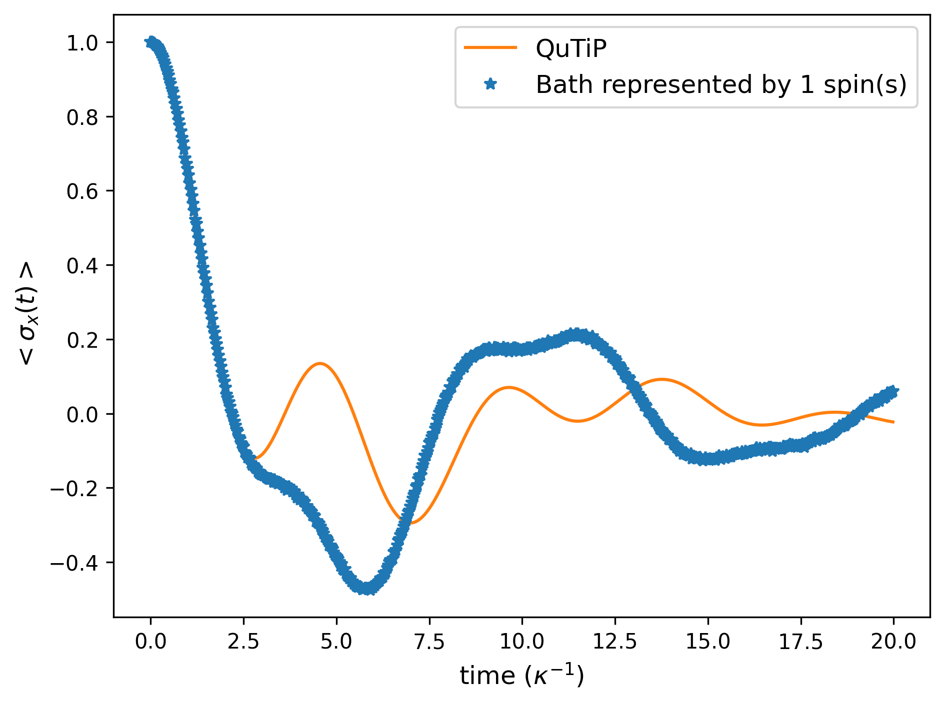
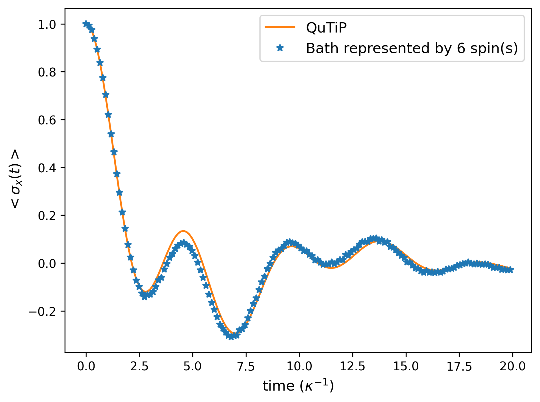
We see that the quantum simulation with 1 spin gives incorrect dynamics, whereas the one with 6 spins shows dynamics which are almost identical to the correct result. The remaining difference is due to the number of bath spins: we can see that the spin bath behaves like one bosonic mode after multiple spins are used to represent it. This result is due to the ultra-strong coupling between the system and bath. The Trotter error is here negligible.

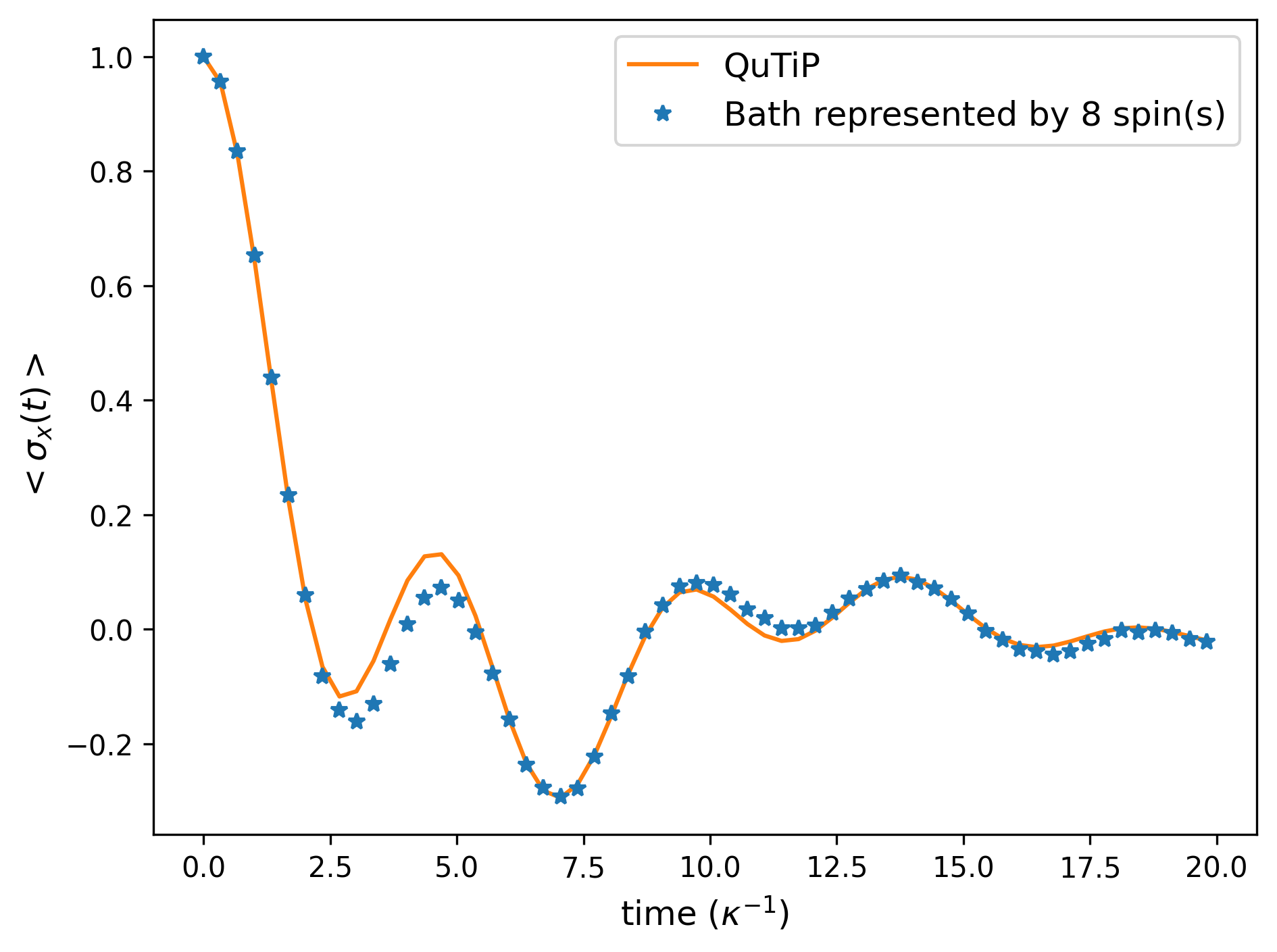
In the next figure, we study the same system, but run the simulation with a non-native gate decomposition (CNOT). Here, we use the bath qubits as control qubits when performing CNOT gates. The simulation is performed for 8 bath qubits.

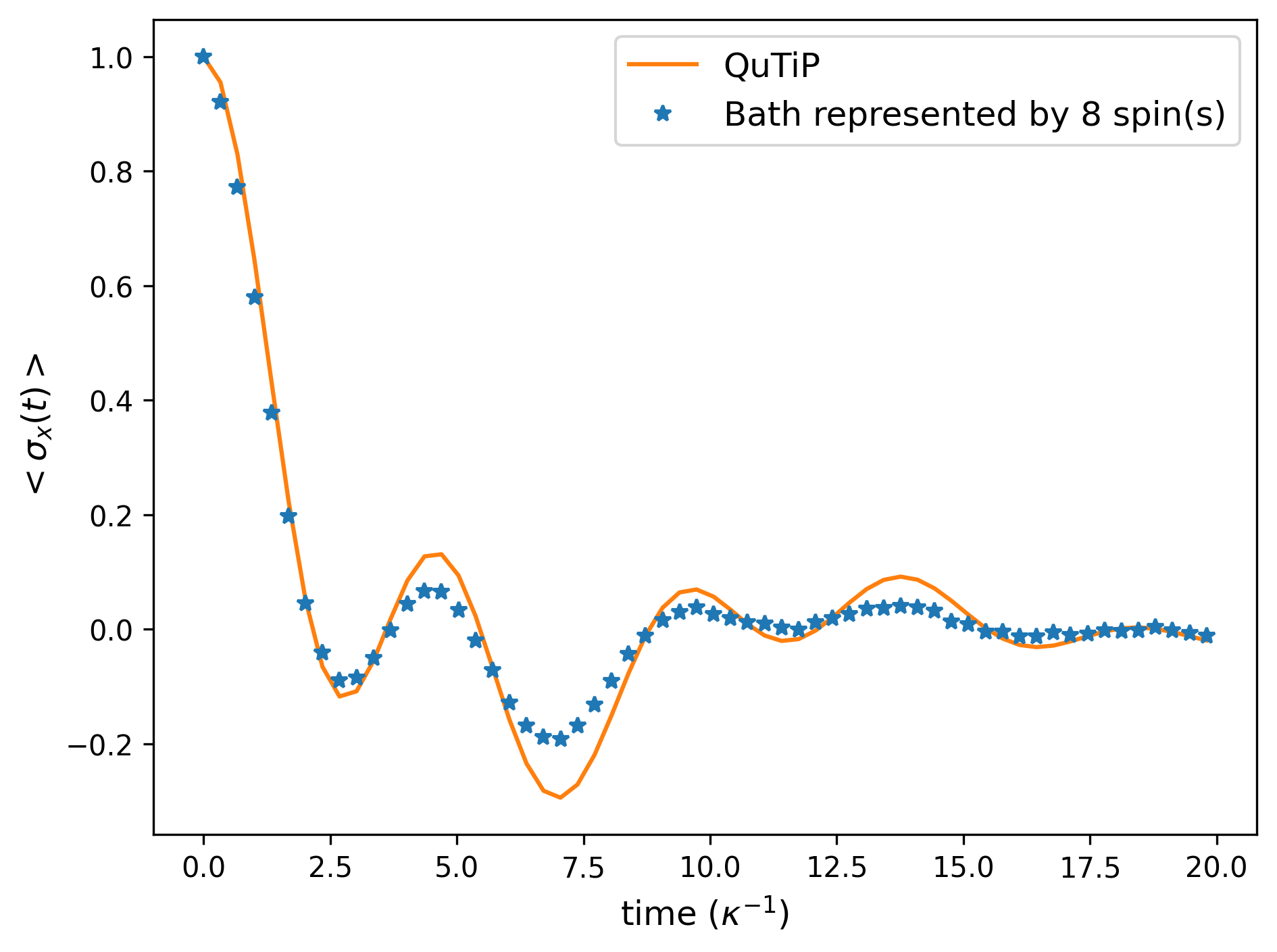
We again find a very small difference between the ideal spin-spin model and the quantum simulation, though now with a marginally larger difference. This is due to a small difference between the ideal and effective noise models. The smallness of the error is still a rather surprising result.

In the last case, we study the CNOT decomposition where the bath qubits are target qubits. The simulation is performed for 8 bath qubits.

Now we can see larger differences in the results. This is due to significant changes in the form of the effective noise. It can be shown that the effective noise model used here includes strong system-qubit dephasing. We then conclude that, in the situations considered, noise-utilising system-bath simulations are feasible and that small changes in gate decompositions can lead to large changes in the effective noise model.

Spin Coupled to an Ohmic Bath

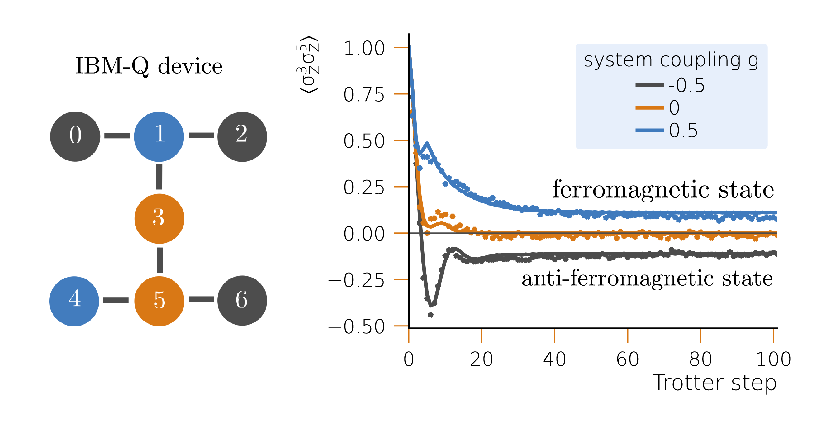
This model is a cornerstone of the spin-boson theory. It shows how system-bath dynamics can change drastically with the strength of the system-bath interaction. Here the strength is characterized by only one parameter \(\alpha\) (the so-called Kondo parameter). As a rough overall picture, for \(\alpha\ll 1\), the system dynamics show damped oscillations, whereas for \(\alpha\lesssim 1/2\), the dynamics transform into slow incoherent relaxation. For \(\alpha > 1\) and \(T=0\) the system does not relax.

Using the system-bath tool, we can demonstrate this transition with a coarse grained bath (at a finite temperature). Below we consider the spectral function:

\[ \begin{align} \Delta &= 1 \\ S(\omega) &= \frac{2\alpha\omega}{1 - \exp(-\omega / T) } \exp(-\vert \omega\vert / \omega_c) \\ \omega_c &= 10 \\ T &= 0.5 \nobreakspace. \end{align} \]

Following our previous procedure, we solve the time evolution when initially prepared in the +1 eigenstate of \(\sigma^x_\textrm{system}\). As a "correct" reference result, we use the so-called NIBA (non-interacting blip approximation) calculation, performing it with the original correct bath and with the coarse-grained baths. (The NIBA calculation is made by a piece of code not provided in the HQS Noise App.) The coarse-graining is performed by optimizing the parameters of 8 bath modes of equal width.

Below, we show the results for quantum simulation with variable-MS decomposition for \( \alpha=0.05 \)

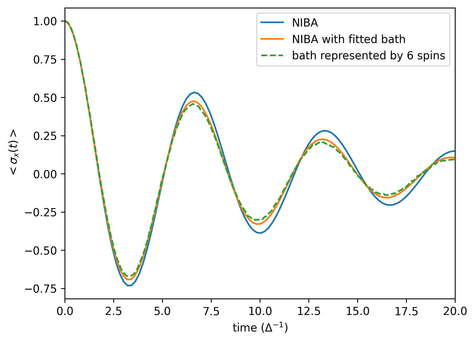
for \(\alpha=0.3\)

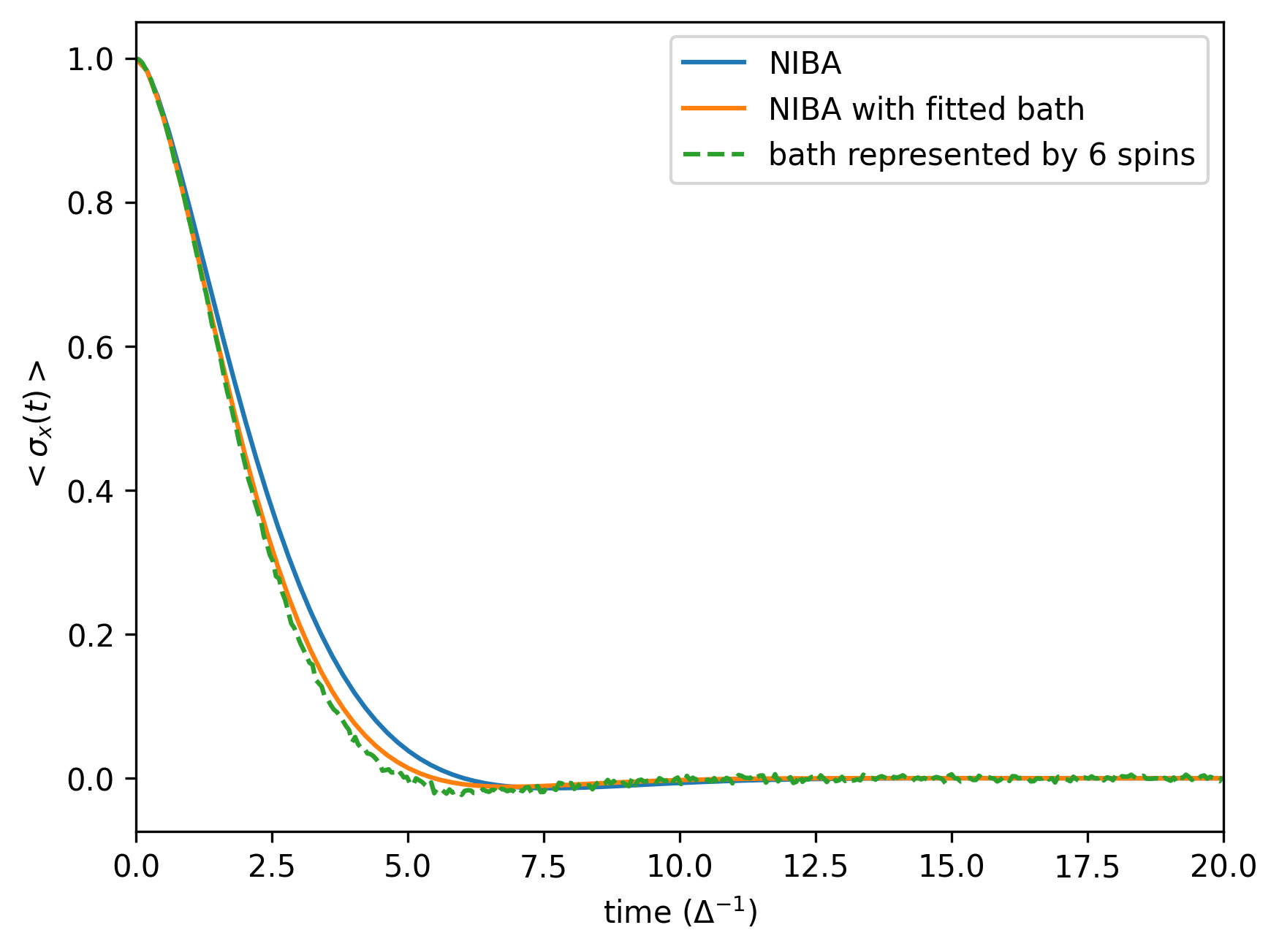
and for \(\alpha=0.6\)

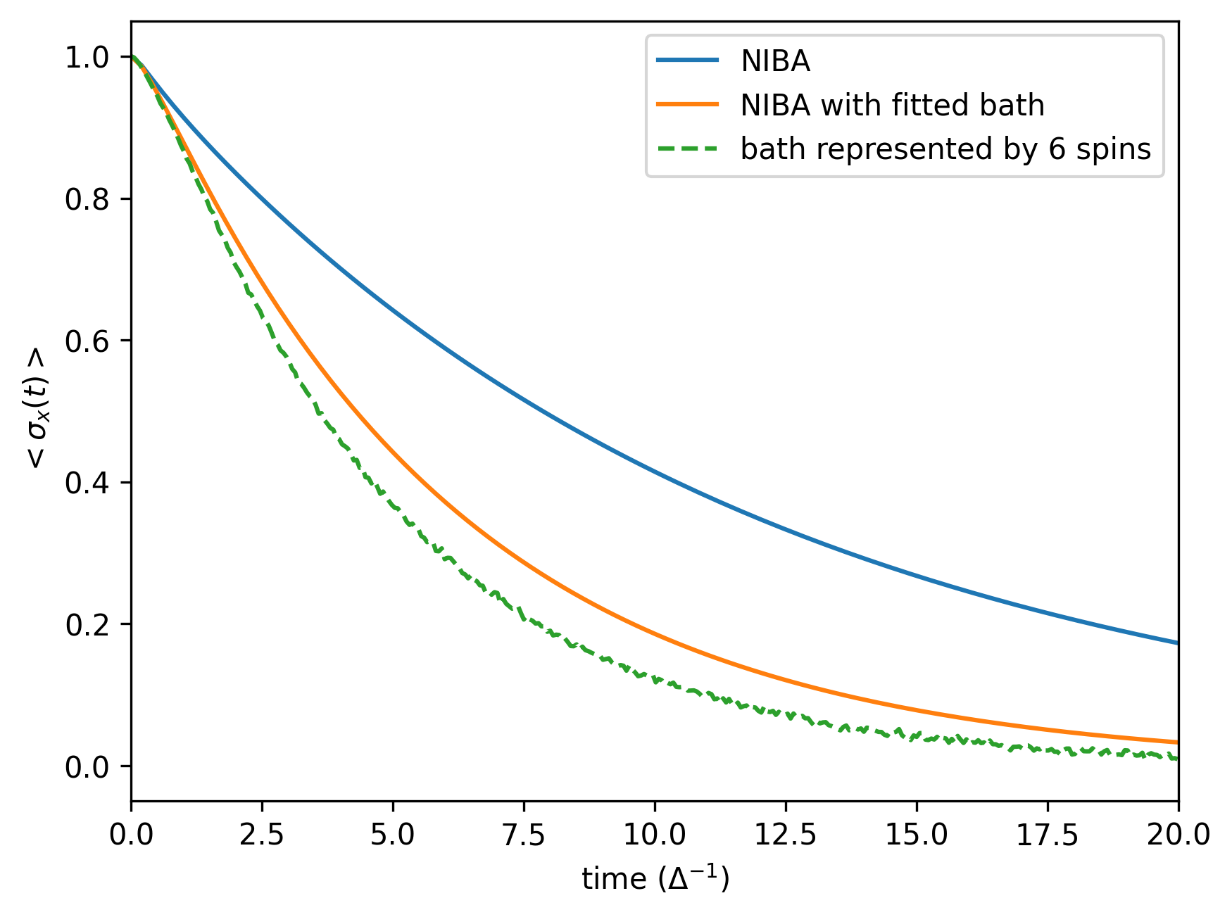
We see the transition from damped oscillations to incoherent decay. The results also agree well with the NIBA solutions. A noticeable difference to the original-bath NIBA result emerges for large \(\alpha\), which is due to an increased sensitivity of dynamics to temperature (the effective coarse-grained bath temperature is increased), rather than an increase in bath-spin populations. As this setup is analogous to the previous example, with the difference of the distributed bath parameters, the conclusions drawn for the CNOT decompositions remain the same.

Exciton Transport

Exciton transport has been studied extensively using multi-spin boson models. The spins correspond to bacteriochlorophyll pigment molecules. Their electronic excited states interact and can effectively "jump" between different sites. They couple longitudinally to a boson bath corresponding to vibrations in the central molecular structure and the surrounding protein. The total Hamiltonian describing this system is of the form:

\[ \begin{align} H &= \sum_{i \in \textrm{system}}\frac{\Delta}{2}\sigma^i_z + \sum_ {i<j \in \textrm{system}} \frac{g_{ij}}{2}\left( \sigma^+_i \sigma^-_j + \sigma^-_j \sigma^+_i \right) \\ &+\sum _{i \in \textrm{system}} \sum _{sm \in \textrm{bath}} \frac{g _{ism}}{2} \sigma^z_i \left[a_s(\omega_m) + a^\dagger_s(\omega_m)\right] + \sum _{sm} \omega_m a^\dagger_s(\omega_m) a_s(\omega_m) \end{align} \] Energy is transferred across a network of 8 spins (or in more general models, 3 sets of 8 spins = 24 spins). This energy transfer occurs with partial energy dissipation in the bath. The environment is often assumed to be Ohmic or sub-Ohmic, but in a more detailed simulation it can be allowed to have more structure. Here, we choose the Ohmic form of a spectral function:

\[ \begin{align} J(\omega) &= \frac{2}{\pi}\frac{\lambda \gamma \omega}{\gamma^2 + \omega^2} \\ \lambda &= 35~\textrm{cm}^{-1} \\ \gamma &= 110~\textrm{cm}^{-1} \\ T &= 100~\textrm{cm}^{-1} (144~K) \nobreakspace . \end{align} \]

and coarse grain it by 2 broad modes. In the simulation, the scaling of the small-angle terms is done exactly in the same way as in the the previous examples. We assume that the noise is purely qubit decay.

Furthermore, we greatly simplify the model and consider here a simplified version of the exciton transport model in photosynthesis: a system of 3 spins with system Hamiltonian:

\[ g_{ij\in\textrm{system}} = \begin{pmatrix} 420 & 95 & 0 \\ & 250 & 30 \\ & & 0 \end{pmatrix} \] These are given in units of \(\textrm{cm}^{-1}\).

The system is initially left to relax to a steady state where there are no excitations in the system. Then an exciton is inserted at site 1 (by \(\sigma^x\) operation). We then monitor the site populations and study how fast the exciton reaches its destination, site 3:

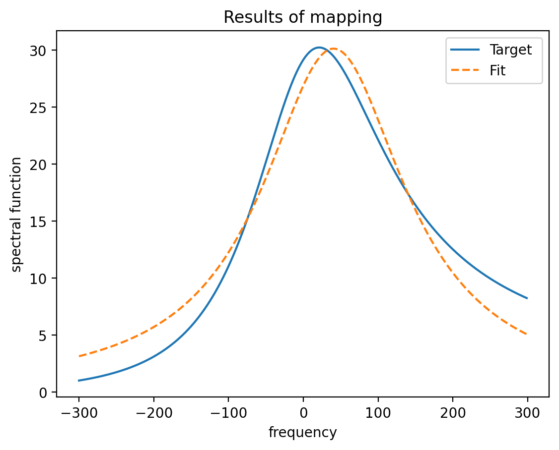
Even though we only include 3 sites in the model here, the result is very similar to those shown in the literature. This agreement despite such a simple model can be rationalized by noting that the number of excited spins in the bath remains low, which is also consistent with the results in the literature.

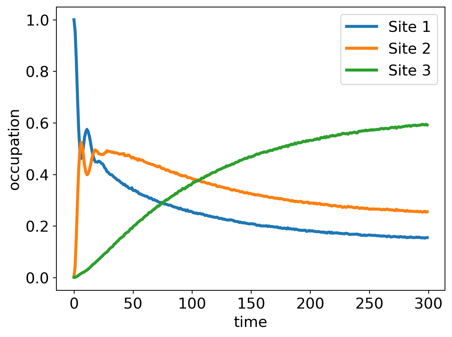
In the second version of the calculation, we add cross-correlations to the system-bath interaction. Specifically, we assume here that half of the spectrum seen by sites 1 and 3 is due to coupling to the bath of site 2. The system-bath coupling of spin 2 remains unchanged, as do the diagonal spectral components of spins 0 and 2.

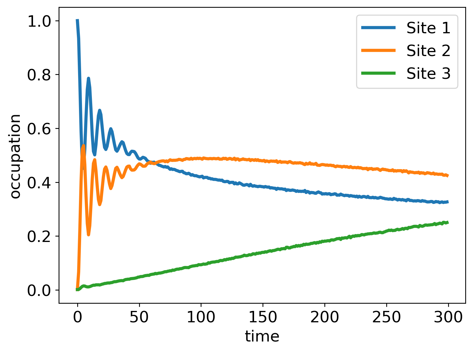
We find relatively strong changes in the solution: the transport to site 3 is essentially weaker. This implies that cross-correlations can be harmful for efficient energy transport. The absence of cross-correlations is indeed the usual assumption taken in numerical simulations.

Changelog

This changelog track changes to the HQS noise app starting at version 0.5.0

0.16.6

• Updated to qonvert 0.14.0.

0.16.5

• Internal workflow fix.

0.16.4

• Updated dependencies.

0.16.3

• Added getters and setters to user documentation.

0.16.2

• Updated to qonvert 0.12.2. Fixes bug relating to routing converter skipping PragmaLoop.
• Fixes bug in SystemBathMSXXAlgorithm when creating a circuit. Set decomposition_blocks setting to true.
• Updated to roqoqo-quest 0.14.4-alpha.3
• Updated to alqorithms 0.13.2-alpha.0
• Switched from using construct_comparison_spin_system to create a circuit for the VariableMSXX system-bath algorithm to using SystemBathMSXXAlgorithm, introduced in alqorithms 0.13.2-alpha.0
• Bugfix for fit_boson_bath_to_spectral_function, where the resampling was failing for some fitting windows. Switched from using self._bath_fitter_resampling to spectral_function.resample, the in-built method for BRNoiseOperators.
• Updated to bath-mapper v0.12.2 (calculate_excitation_spectrum -> calculate_excitation_spectral_function renaming)
• Fixed bug in noisy_algorithm_model and system_bath_noisy_algorithm_model, where the trotter timestep was doubled for the creation of the circuits.
• Fixed bug in create_spin_circuit and create_sysmte_bath_circuit, where the symmetrisation was being applied unnecessarily. This led to the symmetrisation being applied twice in the cases where the normal circuit and symmetrisation circuits were built separately by hand.
• Updated to alqorithms 0.13.1
• Fixed issue ignoring background noise in bath-fitting by upgrading bath-mapper-rs/py to v0.12.2-alpha.1.

0.16.1

• Adds getters/setters to HqsNoiseApp python interface

0.16.0

• Updated to qonvert 0.11.0-alpha.1 which fixes the doubling of DecoherenceOnGateModel bug in "parallelization_blocks" mode.
• Added support for struqture 2.0 inputs, and moved internal logic from struqture 1.0 to 2.0
• Updated licensing package dependency that adds support for unknown entitlements

0.15.3

• Enabling option to use magine-id based license files

0.15.2

• Enabling working with licensefiel obtained by hqstage copy-license

0.15.1

• Update to add support for new entitlements

0.15.0

• Added unroll_quantum_program method that unrolls the symbolic loop inside the QuantumProgram created with the HQS Noise App into a sequence of Trotter timesteps after which each observable is measured. This can only be used with simulator backends and will omit stochastic effects of real measurements and errors in the single layer of basis rotation gates in real measurements.

0.14.5

• Improved error messages for license checks

0.14.4

• Updated text of LICENSE_FOR_BINARY_DISTRIBUTION

0.14.3

• Dependencies update to fix license checks on windows

0.14.2

• Dependencies update to fix license checks on windows

0.14.1

• Update which to dependency libraries fixed bug in creating output registers for measurements

0.14.0

• Bugfix for symmetrization in noisy-algorithm-model

0.13.0

• Activated hqstage license checking

0.12.5

• Update to component libraries

0.12.4

• Internal build release

0.12.3

• Added the estimate_decoherence_rate function

0.12.2

• Deprecated the simulate_quantum_program function and put all simulator tests behind the feature gate for windows support
• Added trotter_step and system_bath_trotter_step functions.
• Added qubit remapping information for bath connectivity.
• Added option to use symmetrization to trotter circuit
• Added option to add wait time to circuit

0.12.1

• Updated to component libraries to support empty coupling when constructing spectra
• Bugfix when fitting procedure tried system bath models with no coupling between system and bath

0.12.0

• Set scipy version to 1.11 due to an issue with qutip (doesn't work with 1.12)
• Fixes bug in construction of mappings for fermion-spin system bath quantum-program construction
• Added truncations for terms below numerical accuracy (1e-14) in fitting results for better stability
• Improved error messages so that users see which algorithms they should choose for which kind of system

0.11.0

• Update to component libraries includin bugfix in measurement preparation (adding wrong MeasureQubit operations)
• Enabled logical-to-physical qubit mappings for system and bath for ParityBased system bath algorithm
• Prepared to use bath-qubit-connectivity information to relax requirement for trilinear chains in when constructing system-bath.

0.11.0-alpha.2

• Update of component libraries

0.11.0-alpha.1

• Fixed double counting of fermionic modes in coupling

0.11.0-alpha.0

• Updated of component libraries

0.10.5

• Updated to qoqo 1.8.0, pyo3 0.20 and update of component libraries

0.10.4

• Fixed serialisation bug
• Updated to component libraries

0.10.3

• Fixed demo build with new options

0.10.2

• Demo version update

0.10.1

• Updated documentation

0.10.0

• Updated to use qoqo NoiseModels

0.9.7

• updated to pyo3 0.19
• Bugfix to noise mapping with system-bath qswap algortihms

0.9.6

• Fixed bug in SWAP algorithm circuit creation using wrong mapping for more than one Trotter step.

0.9.5

• Updated dependencies to qoqo 1.3 struqture 1.1
• Added add_noise function to HQS Noise App for adding device specific noise PRAGMAS to QuantumPrograms

0.9.4

• Updating component libraries, allowing for new single qubit gate sets (pure RotateXY, RotateXY RotateZ and RotateZ SqrtPauliX without InvSqrtPauliX)

0.9.3

• Fixes docstring of noise_mode

0.9.2

• Fixed python dependencies not being installed automatically

0.9.1

• Fixed bug in boson-spin conversion

0.9.0

• Updated to struqture 1.0.0
• Removed deprecated functions
• Updated documentation and ipynb examples
• Fixed minor normalization bug in calculate_excitation_spectrum.

0.8.0

• Switched implementation of calculate_excitation_spectrum to speed up functions.

0.7.0

• Added refactored fitting.py introducing BathFitter class.

0.6.0

• Added support for parallelization_blocks circuits
• Added functions to retrieve circuit depth

0.5.0

• Updated dependencies to component libraries.