System-bath approach
The hqs-noise-app generates algorithms for quantum simulations of system-bath type problems. It is ideal for hardware with one or several good qubits, identified as the system qubits, which have weak noise in comparison to the other qubits, used as bath qubits. This version supports the simulation of spin-boson and spin-fermion systems. The boson or fermion baths are represented by bath spins.
Quick overview
Main idea: utilizing bath-qubit noise
In the HQS approach, noise originating in the bath qubits is effectively filtered and coupled to the system in a way that it appears to come from a bath with a continuous spectral function. This spectral function can be tuned digitally. We optimize the parameters of this system so that it reproduces the spectral function of a given system-bath problem. The optimization is made using a finite number of bath-mode frequencies, system-bath couplings, and bath-mode broadenings. In the quantum simulation, the frequencies and couplings can be implemented digitally. Their magnitude is scaled so that the energy-level broadenings due to the bath noise match to the fitting values. We also provide a SWAP algorithm specifically tailored for system-bath type problems, which takes into account that the bath is non-interacting.
In this version we provide functions to derive constraints for the broadening of the bath qubits from an available device. Providing these constraints to the optimization, the hqs-noise-app will automatically optimize the utilisation of the noisy qubits to improve the simulation results.
Validity
The system-bath simulations are best implemented when:
- system qubits have vanishing or weak noise
- the effective noise of bath qubits is predominantly damping and dephasing
- the quantum computer has a two-dimensional architecture or all-system to all-bath connectivity
These restrictions can, however, be lifted with the cost of reduced simulation accuracy or adding modifications to the system-bath model we simulate. For example, various types of noise mechanisms can be included to be a part of the simulation via changes in the form of the spin-boson Hamiltonian. Also, moderate system noise can be included as a constant background in spectral functions, leading to increased effective temperature.
Using the noise-app
The objective is to take in a system-bath (spin-boson and spin-fermion) model that one wishes to simulate. It is given as a mixed-system object (see also the struqture documentation) and can have a dense spectrum of bath modes or only several broad ones. Important is that it can be turned into a spectral function, which is later coarse-grained by the provided fitting tools. The output will be a coarse-grained spin-boson system with optimized parameters. This system will be then turned into a mixed spin-spin system. The final total system is ideally small enough so that it can be simulated on a quantum computer.
In this process, the fitting tool will also provide the best choice of a Trotter timestep when converting the spin-spin system into a quantum circuit that implements the time-propagation under the spin-spin Hamiltonian. Choosing the right Trotter timestep gives the best possible fit between the open system time evolution and the time propagation on the quantum computer under the influence of physical noise.
Coarse graining mixed Hamiltonians
More detailed, the goal of using the tool is to convert either a spin-boson system system (MixedLindbladOpenSystem) to a spin-spin system (MixedHamiltonian).
The spin-boson system corresponds to a Hamiltonian of type:
\[ H_\textrm{input} = H_\textrm{system} + \frac{1}{2}\sum_{i} \sigma^i_x X_i + \sum_{m} \omega_{m} a^\dagger(\omega_m) a(\omega_m) \nobreakspace , \]
where the coupling between the system and the bath is described by spin-boson operators, where the spin parts are single-spin operators, and bosonic part is a linear operator of the form:
\[ X_i = \sum_{m} g_{im} \left[a(\omega_m) + a^\dagger(\omega_m)\right] \nobreakspace . \]
The bosonic bath is non-interacting and has discretized frequencies \( \omega_m \) and widths \(d\omega_m\equiv \gamma_m\). The widths are identified as boson-mode damping rates, corresponding to lorentzian spectral peaks at their frequencies. All of the bosonic parts can also be given by a spectral function:
\[ S_{ij}(\omega) = 2\pi \sum_{m} g_{im}g_{jm} \delta(\omega-\omega_m + \textrm{i}\gamma_m) \nobreakspace , \]
added with the information of the interaction type, which is in this example \(\sigma_x \).
The final objective is to create a Hamiltonian of class MixedHamiltonian,
with system spins and bath spins of the form:
\[ H_\textrm{output} = H_\textrm{system} + \sum_{i\in\textrm{system}}\sum_{j\in\textrm{bath}} \frac{g_{ij}}{2} \sigma_x^i\sigma_x^j + \sum_{j\in\textrm{bath}} \frac{\epsilon_j}{2} \sigma_z^j \nobreakspace . \]
The first part of the mixed system is the original spin-system. The second part is the effective spin-bath, approximating the behaviour (spectral function) of the original bosonic bath. The broadening of the spin-bath modes is implemented by intrinsic noise of the qubits during the quantum simulation. This can be due to qubit damping and dephasing.
For a detailed technical description of the main functions used in the coarse-graining see the simulation examples.
Creating mixed Hamiltonians and open systems
The system-bath model is defined in the interface as a mixed system. The mixed system can either have two spin subsystems, with the first the system and the second the bath, or one spin system and several boson subsystems. The number of boson subsystems needs to be equal to or smaller than the number of spins in the spin-subsystem. The boson subsystems are used to define the spin-boson problem. The mixed system used in quantum simulations here needs to have exactly two spin subsystems: the first subsystem is the system, the second the bath. Only non-interacting baths are allowed. The corresponding system-bath couplings are limited to products of two Pauli operators.
In the following we create a spin-boson Hamiltonian with struqture_py. Struqture is a library that supports building spin objects, fermionic objects, bosonic objects and mixed system objects that contain arbitrary many spin, fermionic and bosonic subsystems. The struqture documentation contains several examples how to define different kinds of Hamiltonians.
The spin-boson Hamiltonian we create has \(2\) system spins and \(3\) bosons. Each of the system spins is coupled to all of the bosons with the coupling matrix system_bath_couplings. The first part of the script will insert the system energies and the inner-system hopping. The next lines define the boson energies and the noise of the bosons. The last step is the insert the coupling between spins and bosons which are coupled through Pauli-z matrix.
from struqture_py import mixed_systems, spins, bosons
from hqs_noise_app import coupling_to_spectral_function
import numpy as np
import matplotlib.pyplot as plt
plt.rcParams.update({'font.size': 12})

# Set number of system spins.
system_spins = 2
# Set number of boson.
number_bosons = 3

system_energies = [0.1, 0.2]
# Hopping within the system spins.
system_hopping = 0.1

# Use three boson baths.
bath_energies = [0, 1, 2]
bath_broadenings = [0.1, 0.2, 0.3]

# System bath coupling matrix.
system_bath_couplings = [[0.3, 0.1, 0.3], [0.2, 0.4, 0.2]]

# Create a new mixed system with one spin and one boson subsystem.
spin_boson_hamiltonian = mixed_systems.MixedLindbladOpenSystem(
    [system_spins],
    [number_bosons],
    [],
)

# Insert system energies.
for (system, system_energy) in enumerate(system_energies):
    index = mixed_systems.HermitianMixedProduct(
        [spins.PauliProduct().z(system)], [bosons.BosonProduct([], [])], []
    )
    spin_boson_hamiltonian.system_add_operator_product(index, 0.5 * system_energy)

# inserting inner-system hopping (0.5*xx + 0.5*yy)
for system in range(system_spins - 1):
    index_xx = mixed_systems.HermitianMixedProduct(
        [spins.PauliProduct().x(system).x(system + 1)],
        [bosons.BosonProduct([], [])],
        [],
    )
    index_yy = mixed_systems.HermitianMixedProduct(
        [spins.PauliProduct().y(system).y(system + 1)],
        [bosons.BosonProduct([], [])],
        [],
    )
    spin_boson_hamiltonian.system_add_operator_product(index_xx, 0.5 * system_hopping)
    spin_boson_hamiltonian.system_add_operator_product(index_yy, 0.5 * system_hopping)


# Set bath energies
for (bath_index, bath_energy) in enumerate(bath_energies):
    index = mixed_systems.HermitianMixedProduct(
        # Identity spin operator
        [spins.PauliProduct()],
        # Create a Boson occupation operator
        [bosons.BosonProduct([bath_index], [bath_index])],
        [],
    )
    spin_boson_hamiltonian.system_add_operator_product(index, bath_energy)

# Set bath noise
for (bath_index, bath_broadening) in enumerate(bath_broadenings):
    # create the index for the Lindblad terms.
    # We have pure damping
    index = mixed_systems.MixedDecoherenceProduct(
        # Identity spin operator
        [spins.DecoherenceProduct()],
        # Create a Boson occupation operator
        [bosons.BosonProduct([], [bath_index])],
        [],
    )
    spin_boson_hamiltonian.noise_add_operator_product((index, index), bath_broadening)

# Set couplings, use longitudinal (Z) coupling
for spin_index in range(system_spins):
    for (bath_index, system_bath_coupling) in enumerate(
        system_bath_couplings[spin_index]
    ):
        index = mixed_systems.HermitianMixedProduct(
            # Identity spin operator
            [spins.PauliProduct().z(spin_index)],
            # Create a Boson coupling  operator (always a + a^dagger)
            [bosons.BosonProduct([], [bath_index])],
            [],
        )
        spin_boson_hamiltonian.system_add_operator_product(index, system_bath_coupling)


print("Newly created system:")
print(spin_boson_hamiltonian.__repr__())
# create spectrum from Spin-Bath-System
min_frequency = -2
max_frequency = 4
number_frequencies = 1000
frequencies = np.linspace(min_frequency, max_frequency, number_frequencies)

spectrum = coupling_to_spectral_function(spin_boson_hamiltonian, frequencies)

print("Spectrum frequencies")
print(spectrum.frequencies())

print("Spectrum for 0, 0 spin indices with Z coupling")
print(spectrum.get(("0Z", "0Z")))

print("Spectrum for 0, 1 spin indices with Z coupling")
print(spectrum.get(("0Z", "1Z")))
System-bath circuits
We also provide algorithms specifically tailored for system-bath type problems, which take into account that the bath is non-interacting and that large-angle rotations of the bath qubits should be avoided. System-bath interactions can be generated optimally (at least) for two types of hardware connectivity/architechture.
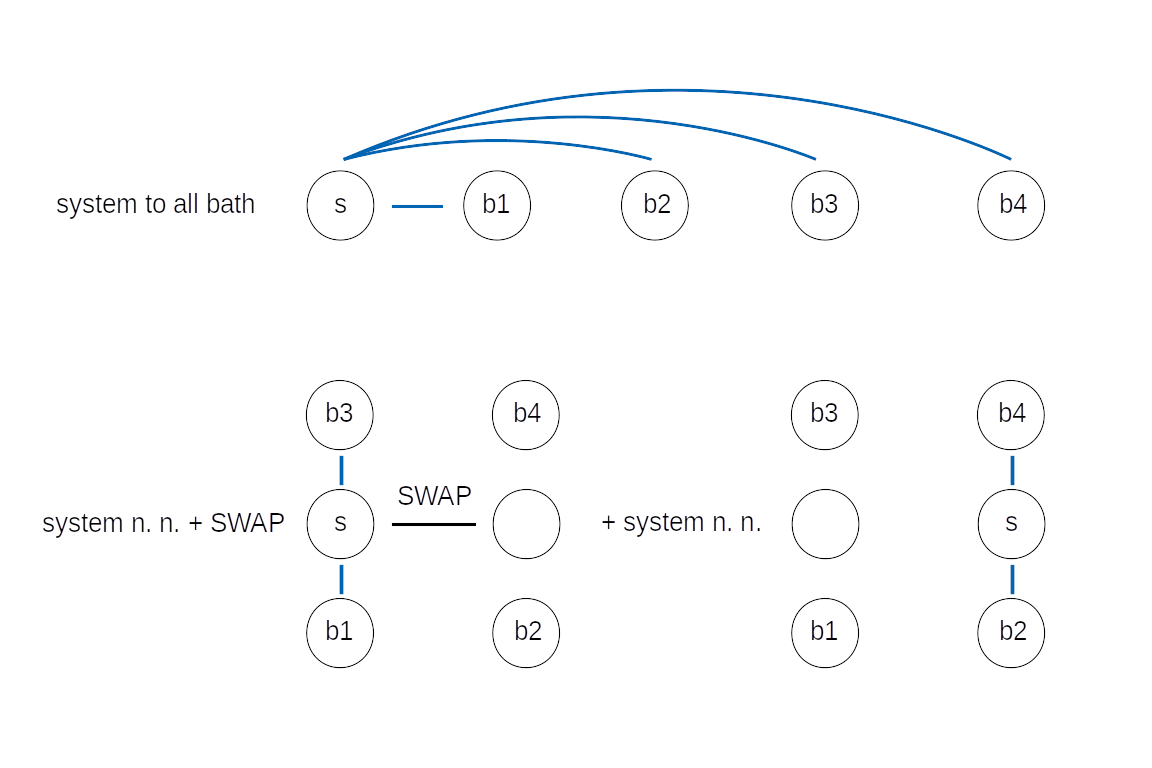
Top: System-bath interactions generated using system to all-bath connectivity. Bottom: System-bath interactions generated in 2d-architecture using nearest-neighbour connectivity and a special SWAP algorithm.
Ideally, all system qubits are connected to all bath qubits.
For system-bath problems connectivity between bath qubits is not needed, since the bath is usually assumed to be non-interacting.
This approach is used when using the algorithm ParityBased (see also the description on page interface).
On the other hand, if only nearest-neighbour interactions are possible,
we offer the user an automatic circuit generation based on a SWAP algorithm specifically optimized for system-bath type problems and 2d hardware-architecture.
Here, the quantum state(s) of the system spin(s) are moved (or swapped) in a system-qubit network, located between the bath qubits.
Within this modification, one avoids performing SWAPs between bath qubits, which can cause major modifications to the effective noise model.
In the example shown above, the state of the spin is stored by two system qubits, one per time.
This architechture most optimally stores a system consisting of \(n\) spins coupled to \(2n\) bath modes.
This approach is used when using the algorithm QSWAP.
The noise-app
The noise-app allows to set properties of the noise model and several other features. A simple example that initialises the noise-app with the noise-mode and the algorithm is
from hqs_noise_app import HqsNoiseApp

# Initialize noise app.
algorithm = "VariableMolmerSorensen"

noise_app = HqsNoiseApp()
noise_app.algorithm = algorithm

# Print all available methods of the HqsNoiseApp
print(dir(HqsNoiseApp))

# Print docstring of algorithm
help(HqsNoiseApp.algorithm)
The available algorithms are
ParityBased: An algorithm that implements the time evolution under a product of PauliOperators via the total Parity of the set of involved qubits.QSWAP: Terms in the Hamiltonian involving two qubits are implemented using a swap network that reorders the terms.QSWAPMolmerSorensen: The QSWAP algorithm using variable angle Mølmer Sørensen XX interaction gates.VariableMolmerSorensen: An algorithm that implements terms in the Hamiltonian involving two qubits with a basis change and variable angle Mølmer Sørensen gates
Besides algorithm, there are several other parameters that can be set with the HqsNoiseApp. A complete list of methods can be obtained with
print(dir(HqsNoiseApp)). Information about the methods can then be obtained by help(HqsNoiseApp.algorithm) for example.
Device and Noise Model
Some of the functions of the noise-app require that we define a device and/or a noise model to run the algorithm. These are defined in qoqo. The documentation contains several examples about how to use qoqo. Important for the noise-app is mainly how to set up a device and create a noise model.
from qoqo import devices, noise_models
# Number of qubits.
number_qubits = 3

# Setting up the device.
single_qubit_gates = ["RotateX", "RotateZ"]
two_qubit_gates = ["VariableMSXX"]

# Same time for all qubits.
gate_time = 1.0

# Setup device with all-to-all connectivity.
device = devices.AllToAllDevice(
    number_qubits, single_qubit_gates, two_qubit_gates, gate_time
)
# Set up a noise model
noise_model = noise_models.ContinuousDecoherenceModel()

# Damping and dephasing of qubits.
qubit_damping_rates = [0.01, 0.02, 0.15]
qubit_dephasing_rates = [0.004, 0.006, 0.12]

# Add damping and dephasing to qubits.
for ii in range(number_qubits):
    noise_model = noise_model.add_damping_rate([ii], qubit_damping_rates[ii])
    noise_model = noise_model.add_dephasing_rate([ii], qubit_dephasing_rates[ii])

# Set single qubit gate times.
for qubit in range(number_qubits):
    device.set_single_qubit_gate_time('RotateX', qubit, 0.03)
    device.set_single_qubit_gate_time('RotateZ', qubit, 0.01)
The above noise model has different rates for all qubits. We also set the gate times for single qubit gates to be faster than the gate times of the two-qubit gate.
System-bath functions
We provide several functions specifically for the system-bath analysis. The following is a list of system-bath functions that are included with the Noise App. Please refer to the documentation of the Bath Fitter for additional system-bath tools.
-
coupling_to_spectral_function: A tool that takes a spin-boson system-bath and creates the effective spectral function seen by the system. The couplings in the system-bath correspond to \(g_{ism}\). If the spectral function is unphysical, the closest solution according to the Frobenius norm is returned.-
Import:
from hqs_noise_app import coupling_to_spectral_function -
Input:
spin_boson_system(MixedLindbladOpenSystem): The struqture system-bath model that contains the couplings and baths from which the spectral function is constructed. The pure system part is ignored for the construction of the spectral fucntion.frequencies(np.ndarray): The spectral function can be constructed for arbitrarynfrequencies. For standard use-cases we recommend using a fine-grained sequence of evenly spaced values e.g. by using :code:np.linspace(start, stop, 1000)as the parameterbackground(float): A constant background shift that is applied to the on-diagonal ((0,0), (1,1) etc.) parts of the spectral function. Can be used to represent direct decoherence on the system-parts of the system-bath model
-
Output:
spectrum(SpinBRNoiseOperatororFermionBRNoiseOperator): Spectral function with cross-correlations. Also contains the frequencies extracted from the coupling in the system-bath hamiltonian.
-
-
spectral_function_to_coupling: The opposite of the previous function. It takes the spectral function seen by a spin system and constructs a collection of bosonic baths that would produce that spectral function. The constructed bosonic baths can include cross-correlations in the coupling. If the spectral function is unphysical, the closest solution according to the Frobenius norm is returned.-
Import:
from hqs_noise_app import spectral_function_to_coupling -
Input:
spectrum(SpinBRNoiseOperatororFermionBRNoiseOperator): Spectral function with cross-correlations. The values of the spectral function are defined for given frequencies.number_spins(int): Number of spins in the system part of the mixed system.
-
Output:
MixedLindbladOpenSystem: The bath and coupling parts of a spin-boson system-bath in the form of a struqtureMixedLindbladOpenSystem. The pure system parts of the model will be empty.
-
-
SpinBRNoiseOperator: A helper class that can represent the spectral function for a spin-system for defined frequencies. Includes cross-correlations.-
Import
SpinBRNoiseOperatorfrom hqs_noise_app import SpinBRNoiseOperator -
Input: -
frequencies(np.ndarray): The frequencies for which the spectral functions are defined. -
Output:
SpinBRNoiseOperator: New empty spin spectrum.
-
Functions:
set(key: (PauliProduct, PauliProduct), spectrum: np.ndarray): Set the component of the spectral function corresponding to the PauliProduct given by key.get(key: (PauliProduct, PauliProduct)): Get the component of the spectral function corresponding to the PauliProduct given by key.frequencies(): Return the frequencies the spectral function is defined for.get_spectral_function_matrix(spectrum_index: int, number_spins: int): Gets the matrix of the spectral function of a spin-system at a specific energy index. A real spectral function needs to be symmetric in the coupling indices. The method will fail if the SpinBRNoiseOperator is not symmetric. The output of this function will be of size3n, as for each index there are three possible coupling types:X,Y, andZ.resample(frequencies: np.ndarray): Resamples the SpinBRNoiseOperator on a new set of frequencies. The SpinBRNoiseOperator defined on the old frequencies is interpolated for the new frequencies. The interpolated values are taken as the new values of the spectral function for these frequencies.
-
-
FermionBRNoiseOperator: A helper class that can represent the spectral function for a spin-system for defined frequencies. Includes cross-correlations.-
Import
FermionBRNoiseOperatorfrom hqs_noise_app import FermionBRNoiseOperator -
Input: -
frequencies(np.ndarray): The frequencies for which the spectral functions are defined. -
Output:
FermionBRNoiseOperator: New empty spin spectrum.
-
Functions:
set(key: (FermionProduct, FermionProduct), spectrum: np.ndarray): Set the component of the spectral function corresponding to the FermionProduct given by key.get(key: (FermionProduct, FermionProduct)): Get the component of the spectral function corresponding to the FermionProduct given by key.frequencies(): Return the frequencies the spectral function is defined for.get_spectral_function_matrix(spectrum_index: int, number_spins: int): Gets the matrix of the spectral function of a spin-system at a specific energy index. A real spectral function needs to be symmetric in the coupling indices. The method will fail if the FermionBRNoiseOperator is not symmetric. The output of this function will be of sizen*n, as for each index there arenpossible coupling types:c^\dagger_0 c_0 ... c^\dagger_0 c_n.resample(frequencies: np.ndarray): Resamples the FermionBRNoiseOperator on a new set of frequencies. The FermionBRNoiseOperator defined on the old frequencies is interpolated for the new frequencies. The interpolated values are taken as the new values of the spectral function for these frequencies.
-
Spin-boson model
In a nutshell
The spin-boson model studies the dynamics of a two-state system interacting with a continuous bosonic bath. Such systems are ubiquitous in nature. Examples include state decay of atoms, certain types of chemical reactions, and exciton transport in photosynthesis.
The great applicability of the spin-boson theory is based on the idea that the bath does not need to be microscopically bosonic, but needs only to behave like one. If an interaction with a bath is mediated by a operator \(Y\), this coupling operator can be replaced by linear bosonic operator \(X\) of a fictitious (non-interacting) bosonic bath, if:
- the coupling is weaker than the bath memory decay, or
- the coupling is strong but statistics of \(Y\) are approximately Gaussian
The corresponding spectral functions then need to match:
\[ \int_{-\infty}^\infty e^{i\omega t} \langle X(t) X(0)\rangle_0 dt = \int_{-\infty}^\infty e^{i\omega t} \langle Y(t) Y(0)\rangle_0 dt \nobreakspace . \]
This is imposed over some relevant frequency range \(\omega_\textrm{min}<\omega<\omega_\textrm{max}\) and "smoothening" \(d\omega\), corresponding to shortest and longest relevant timescales in the problem. Here the subscript-0 refers to an average during free-evolution.
Generally, solving the spin-boson model with numerical methods becomes more difficult when increasing the system-bath couplings as well as the spectral structure.
Hamiltonian, spectral function, and spectral density
The Hamiltonian of the "traditional" spin-boson problem is of the form:
\[ H = \frac{\Delta}{2}\sigma_z + \frac{1}{2}\sigma_x\left[ \epsilon + \sum_i (g_i a_i + g_i^* a^\dagger_i)\right] + \sum_i \omega_i a^\dagger_i a_i \nobreakspace , \]
with possible (trivial) exchange between \(\sigma_z\) and \(\sigma_x\). Here, the two-level system (spin) has a level-splitting \(\Delta\) and a transverse coupling to a bath position-operator:
\[ X=\sum_i g_i a_i + g_i^* a_i^\dagger \nobreakspace . \]
A central role is played by the (free-evolution) bath spectral function:
\[ S(\omega) = \int e^{i\omega t}\left< X(t)X(0)\right> _0 dt \nobreakspace , \] as it fully defines the effect of the bath on the system. In thermal equilibrium, we have:
\[ S(\omega) = \frac{2\pi J(\omega)}{1-\exp\left( -\frac{\omega}{k_{\rm B}T } \right)} \nobreakspace . \] where the spectral density is defined as:
\[ J(\omega) = \sum_i |g_i|^2 \delta(\omega-\omega_i) \quad \omega >0 \nobreakspace , \]
and thereby connects the spectral density to the couplings and frequencies in the Hamiltonian.
Representing a finite temperature bath by a zero-temperature bath
At zero temperature, the spectral function and density differ only by a front factor. It follows that the couplings in the Hamiltonian define the spectral function.
It is possible to represent the spectral function at \(T>0\) by a spectral function of some another system at \(T=0\). For this one needs to introduce negative boson frequencies. We also define \(T=0\) as the situation where all boson modes are empty. The corresponding new Hamiltonian couplings are then defined as:
\[ \sum_i |g_i|^2 \delta(\omega-\omega_i) \equiv \frac{S(\omega)}{2\pi} . \] We use this description of spin-boson systems due to the simplicity it provides, and since it is the description that the final coarse-grained system also corresponds to.
Other forms of the (single) spin-boson Hamiltonians
We can perform a generalization of the "standard" spin-boson model and include several baths coupling via different directions, each of them have their own coupling polarization (X, Y, or Z),
\[ \begin{align} H &= \frac{\Delta}{2}\sigma_z + \frac{1}{2}\sigma_x X + \frac{1}{2}\sigma_y Y + \frac{1}{2}\sigma_z Z \\ &+ \sum_i \omega_{Xi} a^\dagger_{Xi} a_{Xi}+ \sum_i \omega_{Yi} a^\dagger_{Yi} a_{Yi}+ \sum_i \omega_{Zi} a^\dagger_{Zi} a_{Zi} \end{align} \] Here, the spin is coupled to three independent baths.
A model that emerges when mapping electron-transport models to the spin-boson theory is:
\[ \begin{align} H &= \frac{\Delta}{2}\sigma_z + \frac{1}{2}\sigma^+\left( \sum_i g_i (a_{1i} + a^\dagger_{2i})\right) + \frac{1}{2}\sigma^-\left( \sum_i g_i (a^\dagger_{1i} + a_{2i})\right) \\ &+ \sum_i \omega_i \left( a^\dagger_{1i} a_{1i} + a^\dagger_{2i} a_{2i} \right) \nobreakspace . \end{align} \]
Here we have two sets of bosonic environments which have identical parameters. This is a special model since it allows for mapping the system-qubit damping to the bath spectral density.
Generalization to the multi-spin boson model
The above models can be straightforwardly generalized to multi-spin systems. An example is the following Hamiltonian:
\[ \begin{align} H &= \sum_{j \in \textrm{system}}\frac{\Delta}{2}\sigma^j_z + \sum_{jk \in \textrm{system}}\frac{1}{2}\left( g_{jk} \sigma^+_j \sigma^-k + g^*{jk} \sigma^-_j \sigma^+_k \right) \\ &+ \sum {j \in \textrm{system}} \sum {sm \in \textrm{bath}} \frac{1}{2} \sigma^z_j \left[ g{jsm} a_s(\omega_m) + g{jsm}^* a^\dagger_s(\omega_m)\right] + \sum _{sm} \omega_m a^\dagger_s(\omega_m) a_s(\omega_m) \end{align} \]
This is used to describe exciton transport in photosynthesis. The system spins describe the molecular vibrations of excitons and bosonic modes. All excitons couple, in principle, to the same bath. However, such cross-couplings are often neglected. In that case, each exciton has its own bath and we can set \(g_{ism}=0\), if \(i\neq s\).
Spectral function, spectral density, and cross correlations are generalized analogously. In the case of multi-spin-boson model, the spectral function is defined as:
\[ S_{ij}(\omega) = \int e^{i\omega t}\langle X_i(t)X_j(0)\rangle dt \nobreakspace , \] where:
\[ X_i = \sum_{sm} \left[g_{ism} a_s(\omega_m) + g_{ism}^* a^\dagger_s(\omega_m)\right] \nobreakspace , \]
and \(i, j\) refer to system spins. These functions fully define the effect of the bosonic bath on the system. In thermal equilibrium,
\[ S_{ij}(\omega) = \frac{2\pi J_{ij}(\omega)}{1-\exp\left( -\frac{\omega}{k_{\rm B}T } \right)} , , \] where the spectral density is generalized to:
\[ J_{ij}(\omega) = \sum_{sm} g_{ism}^* g_{jsm} \delta(\omega-\omega_m) \quad \omega >0 \] We see that cross-correlations between two spins, elements \(J_{ij}(\omega)\) with \(i\neq j\), can be finite only if different spins couple to the same bath mode.
As in the case of single-spin theory, we model the finite-temperature bath by the corresponding \(T=0\) bath, see section Representing a finite temperature bath by a zero-temperature bath.
Coarse graining details
By "coarse graining", we mean fitting the spectral function using a finite number of broad bosonic modes. It means we limit the number of bath modes to some finite number, but introduce broadenings \(\omega_i\rightarrow\omega_i+\textrm{i}\gamma/2\). A similar approach has been taken in many classical numerical methods, such as in the hierachy of equations of motion (HEOM), or various methods of introducing auxiliary modes with Lindblad decay.
Broad boson modes
Our goal is to construct a bath that reproduces the desired spectral function as well as possible, but includes only a finite number of boson modes. The approach is to make the boson modes broad, so that they effectively represent a continuous bath. Such a broadening can be established theoretically by introducing a damping Lindbladian:
\[ \dot \rho = \textrm{i}[\rho, H] + \gamma\left( a\rho a^\dagger -\frac{1}{2}a^\dagger a\rho -\frac{1}{2}\rho a^\dagger a \right) \nobreakspace . \]
On a Hamiltonian level, the equivalent is to introduce a bilinear coupling between a boson mode and a "flat" environment (bath of the bath). This coupling leads to broadening of spectral peaks,
\[ \begin{align} \langle a(t)a^\dagger\rangle &= e^{-\textrm{i}\omega_0 t - \gamma \vert t \vert/2} \\ \int_{-\infty}^{\infty} e^{\textrm{i}\omega t}\langle a(t)a^\dagger\rangle dt &= 2\pi \frac{1}{\pi}\frac{\gamma/2}{(\gamma/2)^2+(\omega-\omega_0)^2} \end{align} \nobreakspace . \]
Coupling such modes to a system operator such as \(\sigma_z/2\) via a coupling coefficient \(g\) gives the corresponding spectral function peak:
\[ S(\omega) = 2\pi g^2 \frac{1}{\pi}\frac{\gamma/2}{(\gamma/2)^2+(\omega-\omega_0)^2} \nobreakspace . \]
Broad boson modes represented by noisy spins
The coarse-grained bath is bosonic. We aim to represent this using a spin bath. Various efficient "digital" (such as binary or unary) mappings between qubit states and boson states have been proposed in recent literature. However, such encodings do not map the decay of (arbitrary) bath qubits to single-boson annihilation,which is the key correspondence in our approach.
The spin-boson simulator instead directly replaces the coarse-grained bath operators by spin-bath operators, in the simplest case by doing the following:
\[ \begin{align} g(a + a^\dagger) &\rightarrow g \sigma_x \\ \omega a^\dagger a &\rightarrow \frac{\omega}{2}\sigma_z \\ \sqrt{\gamma} a &\rightarrow \sqrt{\gamma}\sigma^- \end{align} \]
This can work, since spins can (collectively) behave like a bosonic field. The condition for this being true boils down to the requirement of coupling-operator statistics to be Gaussian, up to some relevant order. This is clearly valid for a spin-bath with a fast memory decay compared to the system-bath coupling, \(\gamma\gg g\), since here only two-operator correlation functions matter. A less trivial example is a group of identical spins, which can collectively behave like one bosonic mode with long memory time. Such a system is studied explicitly in example XXX.
More generally, we do not have to assume that the spins are identical. A central condition for the bath being bosonic is that individual bath spins are only weakly excited,
\[ \left< \sigma^+_i \sigma^-_i \right> _{\textrm{full solution}} \ll 1 \quad i\in \textrm{bath} \nobreakspace . \]
Note that the collective excitation number, \( \sum_{i\in \textrm{bath}}\left< \sigma^+_i \sigma^-_i \right> _\textrm{full solution}\), can still be fairly large. This relation should be valid for all times during the simulation. It can be probed by bath-qubit measurements.
If the demand is not respected, the "bosonicity" of the bath can be improved by representing a problematic mode by \(N \) spins, all of them with a down-scaled coupling:
\[ g \rightarrow \frac{g}{\sqrt{N}} \nobreakspace . \]
The down-scaling guarantees that the the total spectral function stays unchanged. We then use:
\[ \begin{align} g(a + a^\dagger) &\rightarrow \sum_{i=1}^N \frac{g}{\sqrt{N}} \sigma^x_i \\ \omega a^\dagger a &\rightarrow \sum_{i=1}^N \frac{\omega}{2}\sigma^z_i \\ \sqrt{\gamma}a & \rightarrow \sum_{i=1}^N \sqrt{\gamma}\sigma^-_i \end{align} \] It should be noted that it can also be enough to just increase the total number of broad modes in the spectral-function fitting range (keeping \(N=1\)).
In the coarse-graining theory, the broadening of the bosonic modes is always due to damping. However, the corresponding broadening of the spin modes can also be partly due to dephasing. The correspondence between the broadenings is straightforward:
\[ \gamma = \gamma_\textrm{damping} + \gamma_\textrm{dephasing} \nobreakspace . \]
Noiseless system
In the fitting, our target function is the frequency-discretized multi-dimensional spectral function:
\[ S_{ij}(\omega_m) \equiv S[i, j, m] , . \] It is spin-exchange symmetric, so \(S_{ij}(\omega_m)= S_{ji}(\omega_m)\). More generally, it is Hermitian, as we are dealing with complex couplings.
Our fitting finds an approximation of this function by replacing the original bath by \(n_\textrm{lorentzians}\) broad modes. Each broad mode has a central frequency \(\omega_k\), coupling to the \(i^\text{th}\) spin \(g_{ik}\), and width \(\gamma_k\). The (multi-dimensional) spectral function that follows is:
\[ S_{ij}^\textrm{cg}(\omega) = 2\pi\sum_{k=1}^{n_\textrm{lorentzians}} g_{ik}g_{jk}^*\frac{1}{\pi}\frac{\gamma_k/2}{(\gamma_k/2)^2+(\omega-\omega_k)^2} \nobreakspace . \] The current fitting routine optimizes the following cost function:
\[ C= \sum_{i\leq j} \left \lbrace\sum_k \left [S_{ij}^\textrm{cg}(\omega_k) - S_{ij}(\omega_k) \right]^2 \right \rbrace \nobreakspace , \]
by seeking the optimal values of \(\omega_k\), \(g_{ik}\), and \(\gamma_k\), starting from some initial guess. The general fitting problem then has \(n_\textrm{lorentzians}\) frequencies, \(n_\textrm{spins} \times n_\textrm{lorentzians}\) couplings, and \(n_\textrm{lorentzians}\) widths.
The fitting can also be done using the same broadening for all modes, \(\gamma_m=\gamma\). This can be a more realistic choice when mapping to hardware properties.
Note that if \(n_\textrm{spins}=1\), we are dealing with fitting only one function, \(S_{ij}(\omega_m) \equiv S(\omega_m)\). Furthermore, if \(n_\textrm{spins}>1\), but cross-correlations are very small and diagonal entries (\(i=j\)) of the spectrum are almost identical, it is recommended to do a comparison to the result of fitting the corresponding single-spin systems only.
Open system
We also allow the user to add system-qubit noise as a background to the spectral function and do the fitting with this taken into account. This is motivated by the possibility to add system damping exactly to fermion-transport models. We then introduce a system rate that is an average of bath rates, times some given factor \(f\),
\[ \gamma_\textrm{system} \equiv f \langle \gamma_i\rangle , , \]
and change the spectral function as:
\[ S_{ij}^\textrm{cg}(\omega) = 2\pi\sum_{k=1}^{n_\textrm{lorentzians}} g_{ik}g_{jk}^*\frac{1}{\pi}\frac{\gamma_k}{(\gamma_k/2)^2+(\omega-\omega_k)^2} + \delta_{ij} \gamma_\textrm{system} \nobreakspace . \]
The noise of different system qubits is assumed to be uncorrelated, hence the multiplication by \(\delta_{ij}\). The correct factor \(f\) to be used depends on the model one considers (as well as on hardware properties). Note that the fitting problem stays essentially the same.
Spectral function to coupling
Here, we assume that a spectral function is given as an input and we want to write down a Hamiltonian that reproduces it: we need to solve the system-bath couplings from the spectral function. The spectral function was discretized to frequencies \(\omega_m\), and the corresponding data values are \(S_{ij}(\omega_m)\equiv S[i, j, m]\). In the corresponding Hamiltonian description, the frequencies of the bath modes are going to be \(\omega_m\). It should be noted that if the given spectral function is unphysical, the software will find the closest physical solution (according to the Frobenius norm).
In the case of single-spin system, the couplings will be defined by the areas:
\[ S(\omega_m) d\omega_m = |g_m|^2 \nobreakspace , \]
where \(d\omega_m\) is the width of the frequency interval corresponding to mode \(\omega_m\). The couplings are then solved to be \(g_m=\pm\sqrt{S(\omega_m) d\omega_m}\). Here, the chosen sign is not important.
In the case of \(n\) system spins, the couplings are constructed similarly with the help of linear algebra. We introduce \(n\) bath-submodes per frequency and solve:
\[ S[i, j, m] d\omega_m = \sum_{s=1}^{n} g[i, s, m] g*[j, s, m] \nobreakspace . \]
Here \(g[i, s, m]\) is the coupling from spin \(i\) to bath submode \(s\) at frequency \(\omega_m\). The spectral function is Hermitian with respect to changing \(i\) and \(j\). There are multiple solutions to this equation, some of them having unreasonable and complicated cross-couplings. To find a reasonable solution, we can require:
\[ g[i, s, m] = 0 \qquad \textrm{for } i < s \ . \] In this form, the obtained cross-couplings are zero if there are no spectral-function cross-correlations. The solution can then be found by Cholesky decomposition:
\[ S[:, :, m] = L L^\dagger \ , \] where \(L\) is the solution for the coupling matrix at frequency \(\omega_m\).
If the given spectral function is unphysical (or is rank-deficient), this has no solution. In this case, the software will use an eigendecomposition to find the closest physical solution to \(L\) according to the Frobenius norm.