Examples
In this section, we use the system-bath tool to solve the dynamics of some simple system-bath problems and study the quality of the corresponding quantum simulation. Notebooks with the examples are available in the examples repository of the HQS Noise App.
Spin Coupled to Broad Bosonic Mode
We first look at a system that is coupled to a single bosonic mode and is described by the Hamiltonian
The coupling to the bosonic mode is ultrastrong, . This makes the representation of the bath using spins challenging, but not impossible. Below is a demonstration of how the bosonic bath can be represented by a spin bath. We assume the following: the system qubit is noiseless, the bath qubit noise is due to decay and dephasing, and the noise is always "on".
For each Trotter step, we must correctly scale the phases of the digitally implemented small-angle gates so that the physical broadening matches with the model broadening. For example, we need to fix the phase of the system-bath coupling so that:
where is the circuit depth. It accounts for the accumulation of the noise. The parameter is then used to quantify the total infidelity of one Trotter step.
To demonstrate the possibility of including dephasing on the bath qubit in the effective broadening, we consider the case where the bosonic mode broadening is reproduced by an equal contribution from qubit decay and dephasing ,
Furthermore, we consider the parameters:
We also use , which is a relatively high value, but still does not lead to a noticeable Trotter error. The larger this parameter is, the more Trotter error the quantum simulation will have.
Below, we show a comparison between the exact spin-boson model and the quantum simulation for the (native) variable MS-decomposition, where the bath is described by either 1 spin or 6 identical spins. The simulation starts with the system spin in the +1 eigenstate of operator and the bath in its ground state. We track the time evolution of .
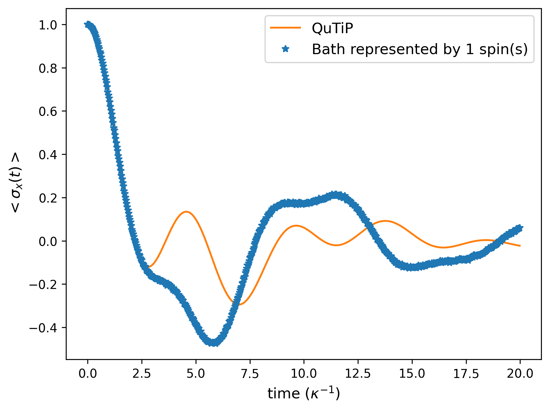
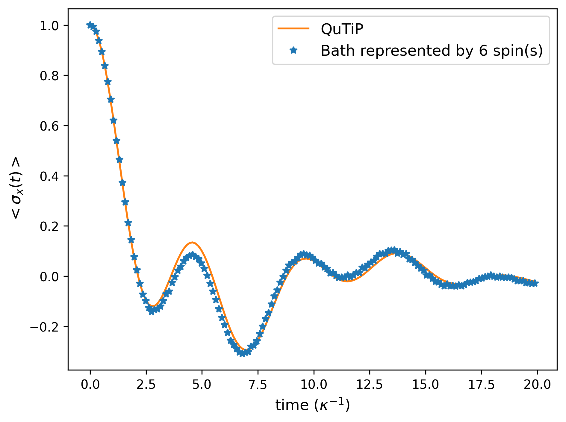
We see that the quantum simulation with 1 spin gives incorrect dynamics, whereas the one with 6 spins shows dynamics which are almost identical to the correct result. The remaining difference is due to the number of bath spins: we can see that the spin bath behaves like one bosonic mode after multiple spins are used to represent it. This result is due to the ultra-strong coupling between the system and bath. The Trotter error is here negligible.
In the next figure, we study the same system, but run the simulation with a non-native gate decomposition (CNOT). Here, we use the bath qubits as control qubits when performing CNOT gates. The simulation is performed for 8 bath qubits.
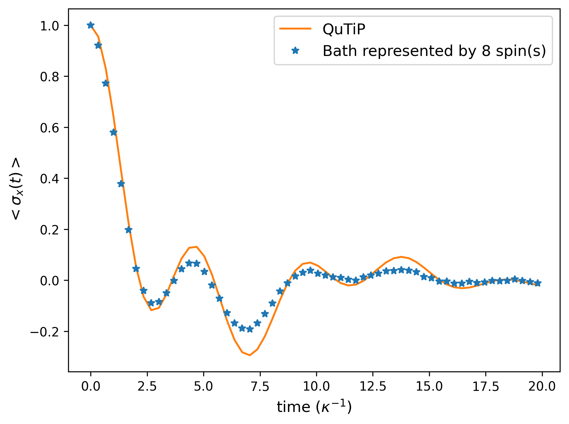
We again find a very small difference between the ideal spin-spin model and the quantum simulation, though now with a marginally larger difference. This is due to a small difference between the ideal and effective noise models. The smallness of the error is still a rather surprising result.
In the last case, we study the CNOT decomposition where the bath qubits are target qubits. The simulation is performed for 8 bath qubits.
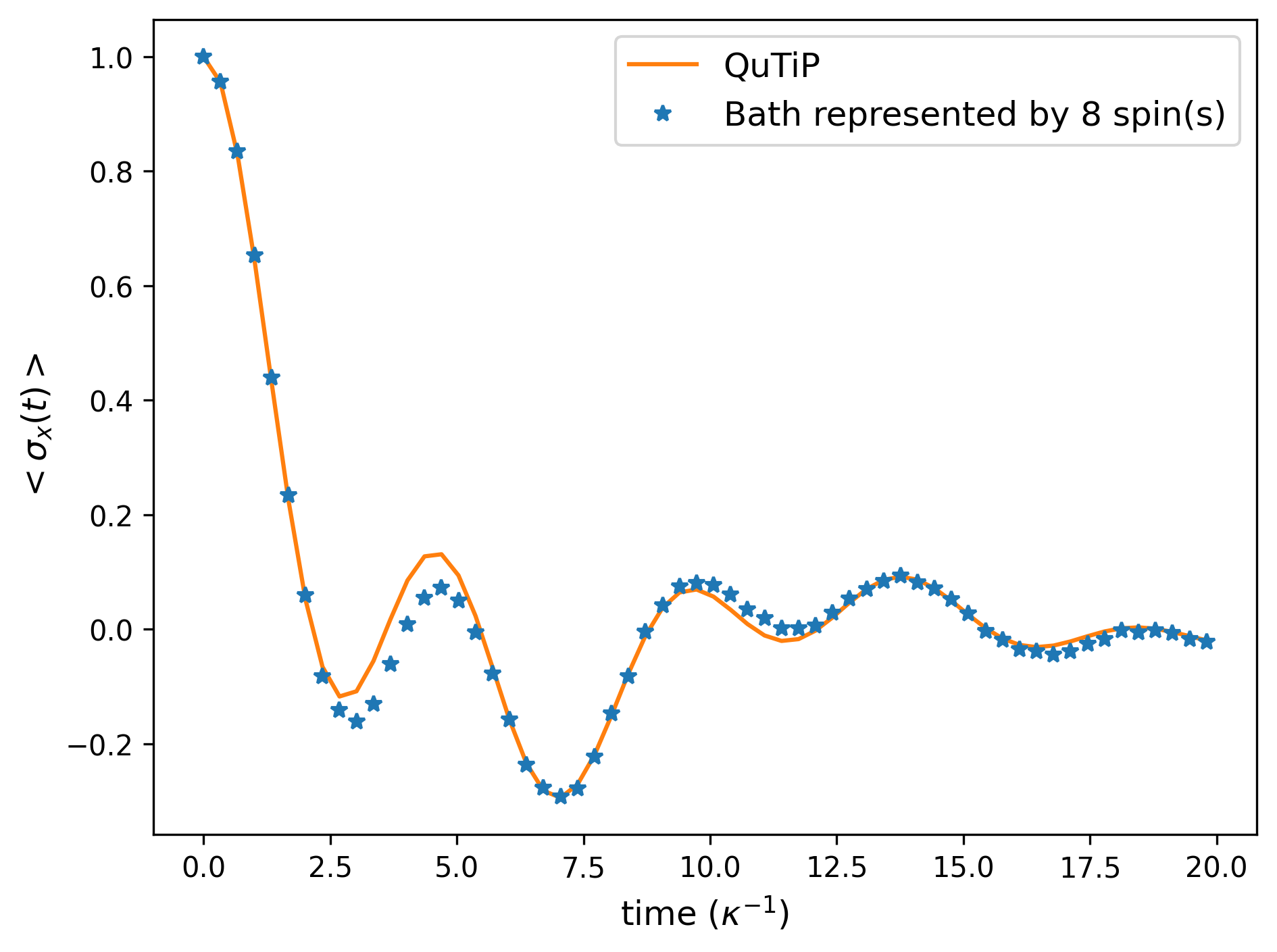
Now we can see larger differences in the results. This is due to significant changes in the form of the effective noise. It can be shown that the effective noise model used here includes strong system-qubit dephasing. We then conclude that, in the situations considered, noise-utilising system-bath simulations are feasible and that small changes in gate decompositions can lead to large changes in the effective noise model.
Spin Coupled to an Ohmic Bath
This model is a cornerstone of the spin-boson theory. It shows how system-bath dynamics can change drastically with the strength of the system-bath interaction. Here the strength is characterized by only one parameter (the so-called Kondo parameter). As a rough overall picture, for , the system dynamics show damped oscillations, whereas for , the dynamics transform into slow incoherent relaxation. For and the system does not relax.
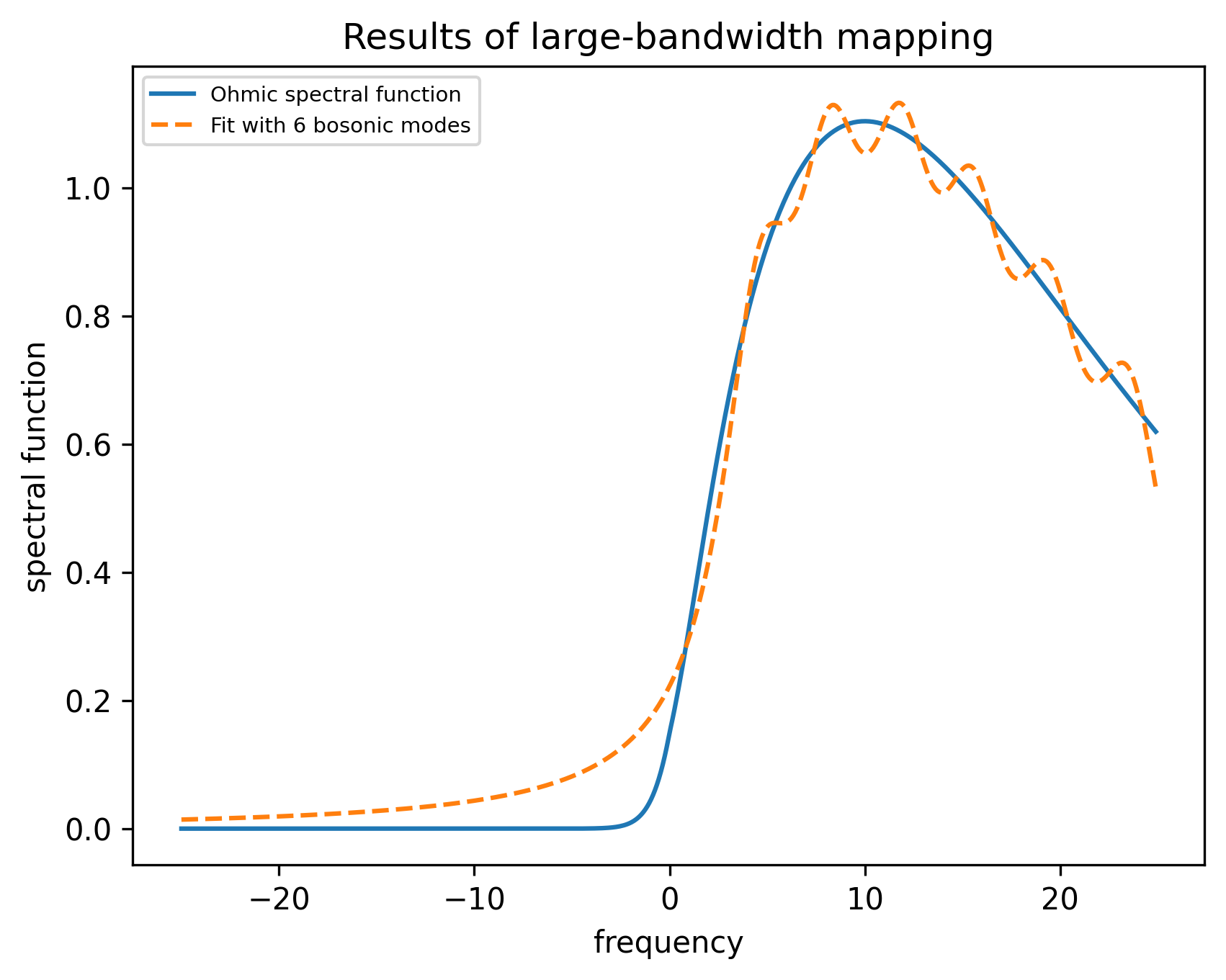
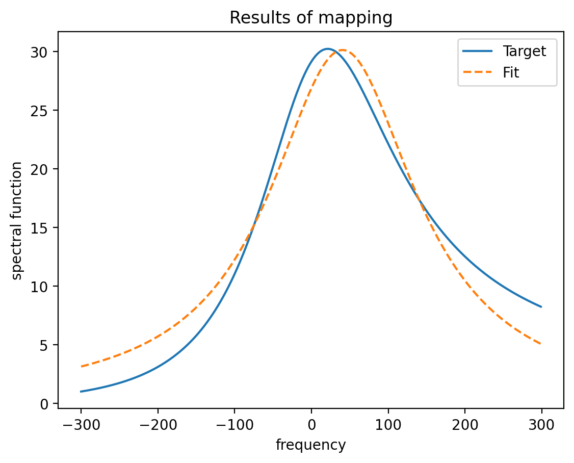
Using the system-bath tool, we can demonstrate this transition with a coarse grained bath (at a finite temperature). Below we consider the spectral function:
Following our previous procedure, we solve the time evolution when initially prepared in the +1 eigenstate of . As a "correct" reference result, we use the so-called NIBA (non-interacting blip approximation) calculation, performing it with the original correct bath and with the coarse-grained baths. (The NIBA calculation is made by a piece of code not provided in the HQS Noise App.) The coarse-graining is performed by optimizing the parameters of 8 bath modes of equal width.
Below, we show the results for quantum simulation with variable-MS decomposition for
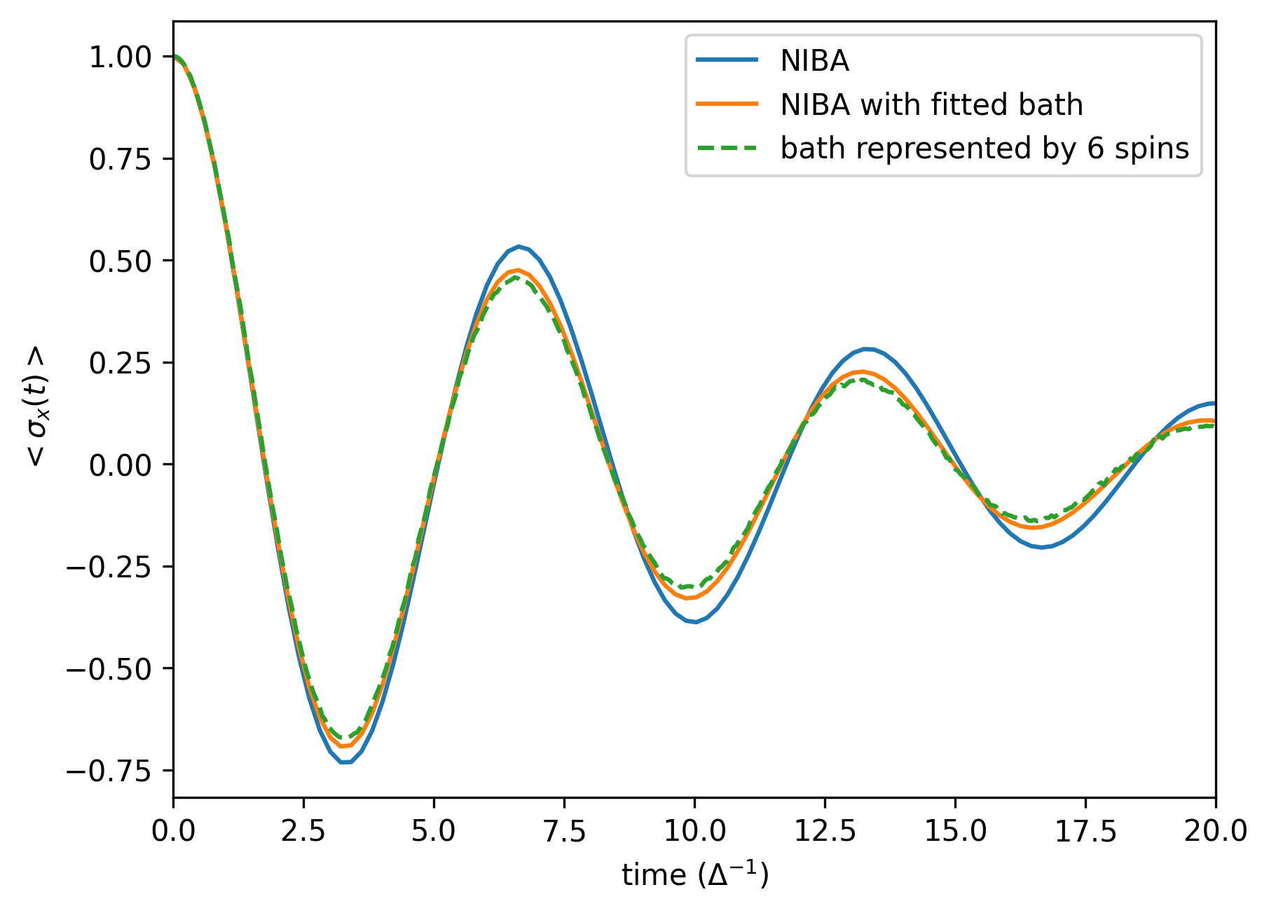
for
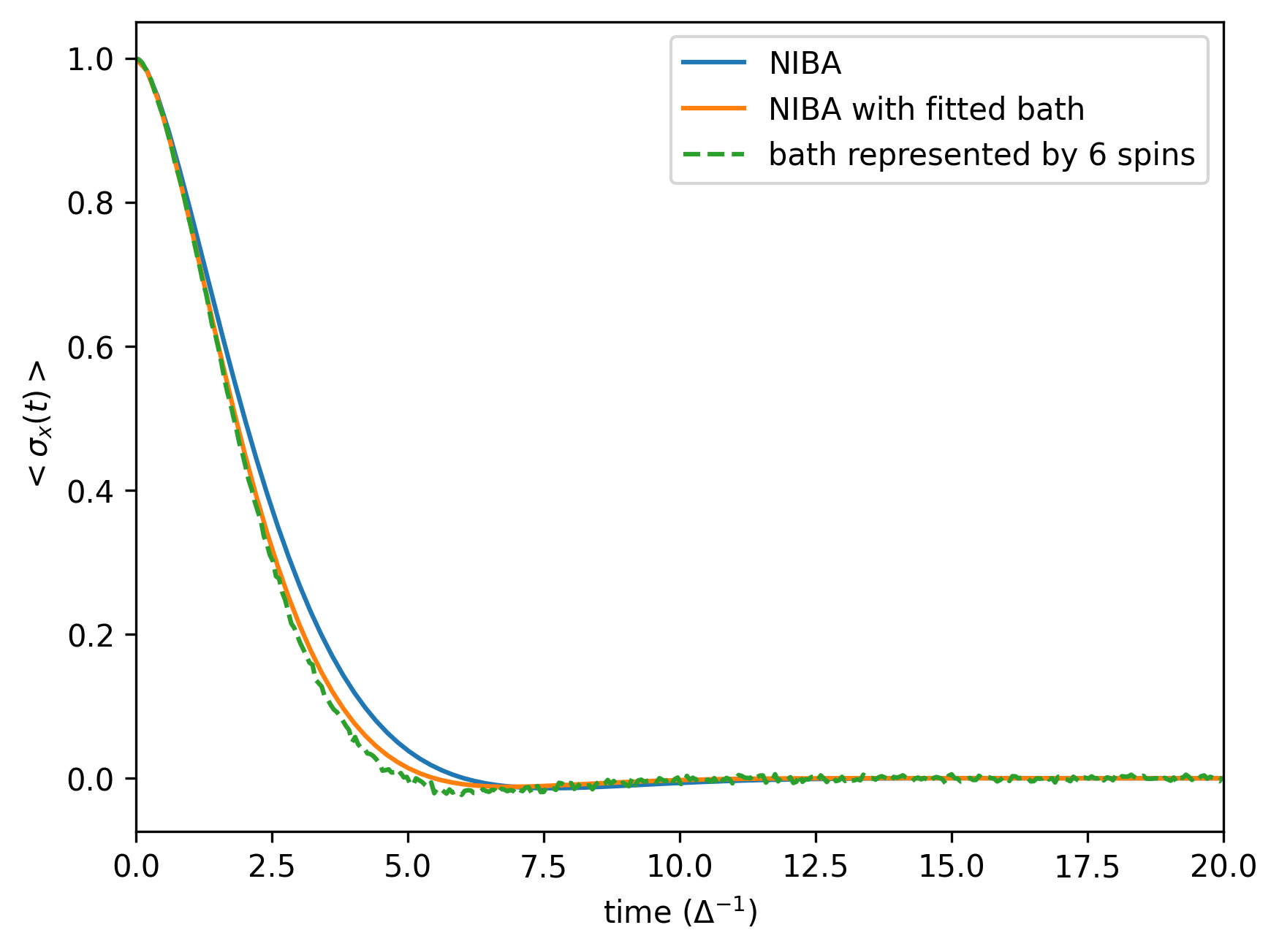
and for
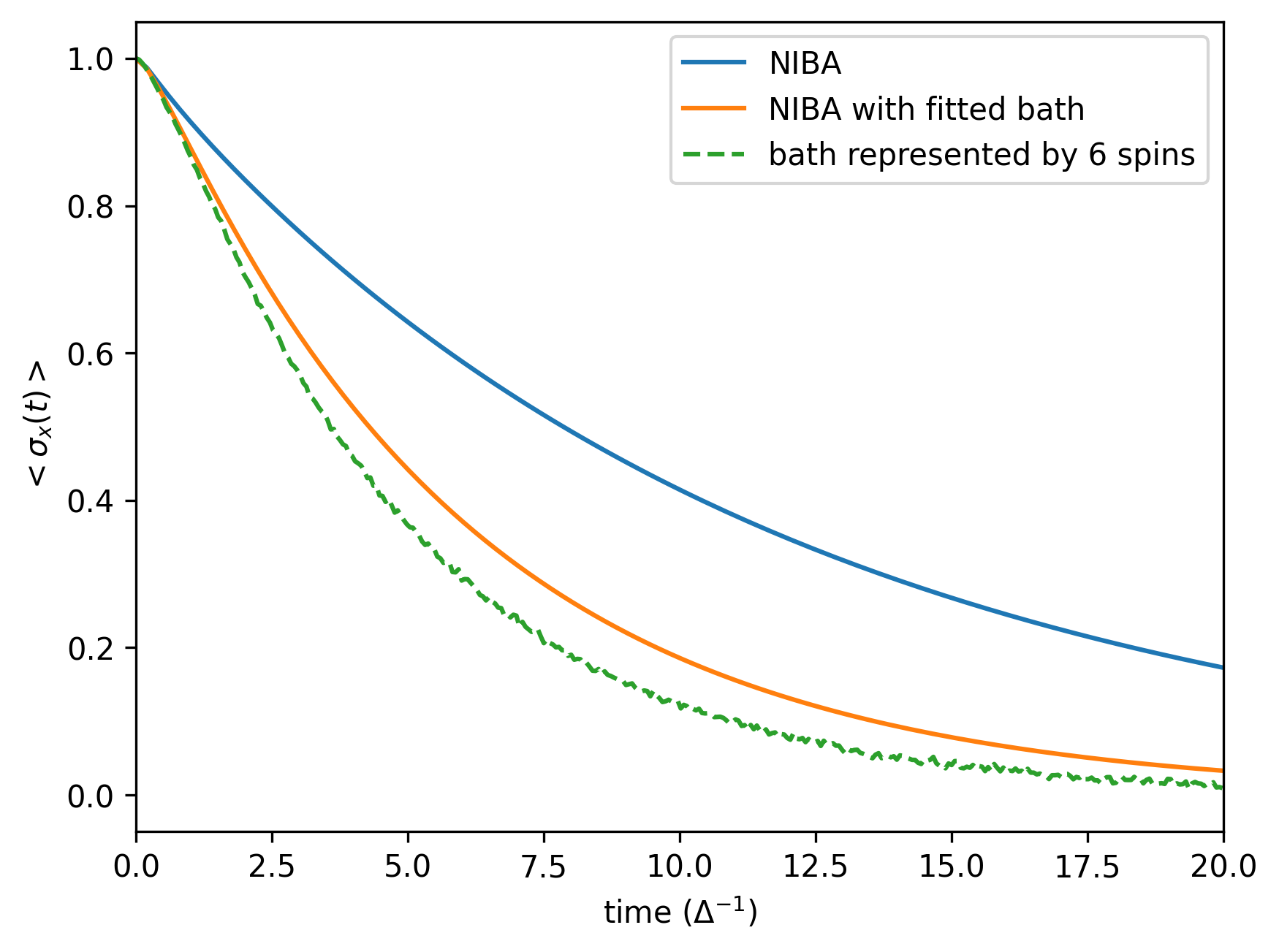
We see the transition from damped oscillations to incoherent decay. The results also agree well with the NIBA solutions. A noticeable difference to the original-bath NIBA result emerges for large , which is due to an increased sensitivity of dynamics to temperature (the effective coarse-grained bath temperature is increased), rather than an increase in bath-spin populations. As this setup is analogous to the previous example, with the difference of the distributed bath parameters, the conclusions drawn for the CNOT decompositions remain the same.
Exciton Transport
Exciton transport has been studied extensively using multi-spin boson models. The spins correspond to bacteriochlorophyll pigment molecules. Their electronic excited states interact and can effectively "jump" between different sites. They couple longitudinally to a boson bath corresponding to vibrations in the central molecular structure and the surrounding protein. The total Hamiltonian describing this system is of the form:
Energy is transferred across a network of 8 spins (or in more general models, 3 sets of 8 spins = 24 spins). This energy transfer occurs with partial energy dissipation in the bath. The environment is often assumed to be Ohmic or sub-Ohmic, but in a more detailed simulation it can be allowed to have more structure. Here, we choose the Ohmic form of a spectral function:
and coarse grain it by 2 broad modes. In the simulation, the scaling of the small-angle terms is done exactly in the same way as in the the previous examples. We assume that the noise is purely qubit decay.
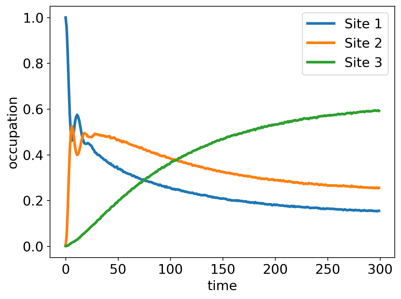
Furthermore, we greatly simplify the model and consider here a simplified version of the exciton transport model in photosynthesis: a system of 3 spins with system Hamiltonian:
These are given in units of .
The system is initially left to relax to a steady state where there are no excitations in the system. Then an exciton is inserted at site 1 (by operation). We then monitor the site populations and study how fast the exciton reaches its destination, site 3:
Even though we only include 3 sites in the model here, the result is very similar to those shown in the literature. This agreement despite such a simple model can be rationalized by noting that the number of excited spins in the bath remains low, which is also consistent with the results in the literature.
In the second version of the calculation, we add cross-correlations to the system-bath interaction. Specifically, we assume here that half of the spectrum seen by sites 1 and 3 is due to coupling to the bath of site 2. The system-bath coupling of spin 2 remains unchanged, as do the diagonal spectral components of spins 0 and 2.
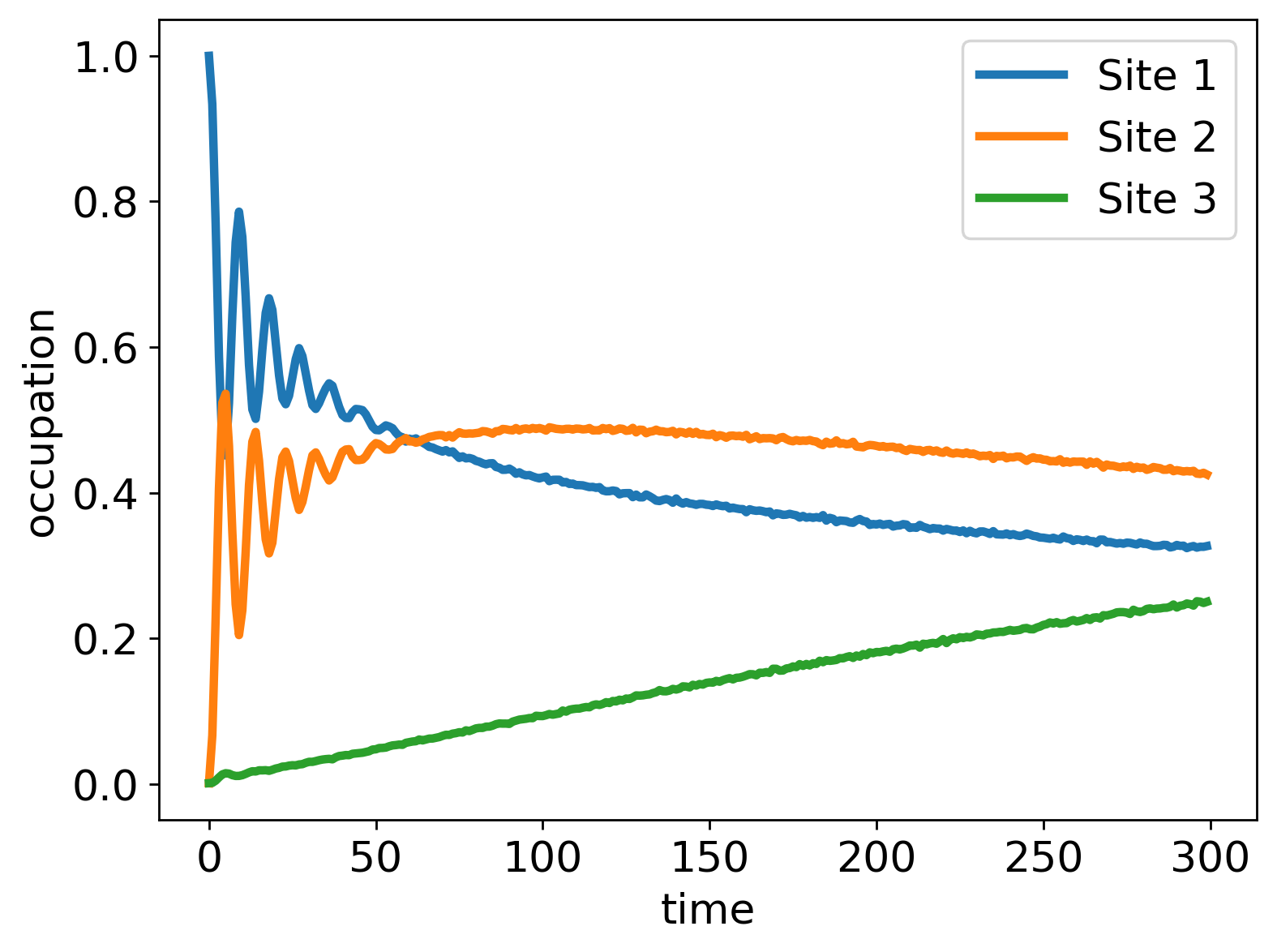
We find relatively strong changes in the solution: the transport to site 3 is essentially weaker. This implies that cross-correlations can be harmful for efficient energy transport. The absence of cross-correlations is indeed the usual assumption taken in numerical simulations.