Lattice Builder
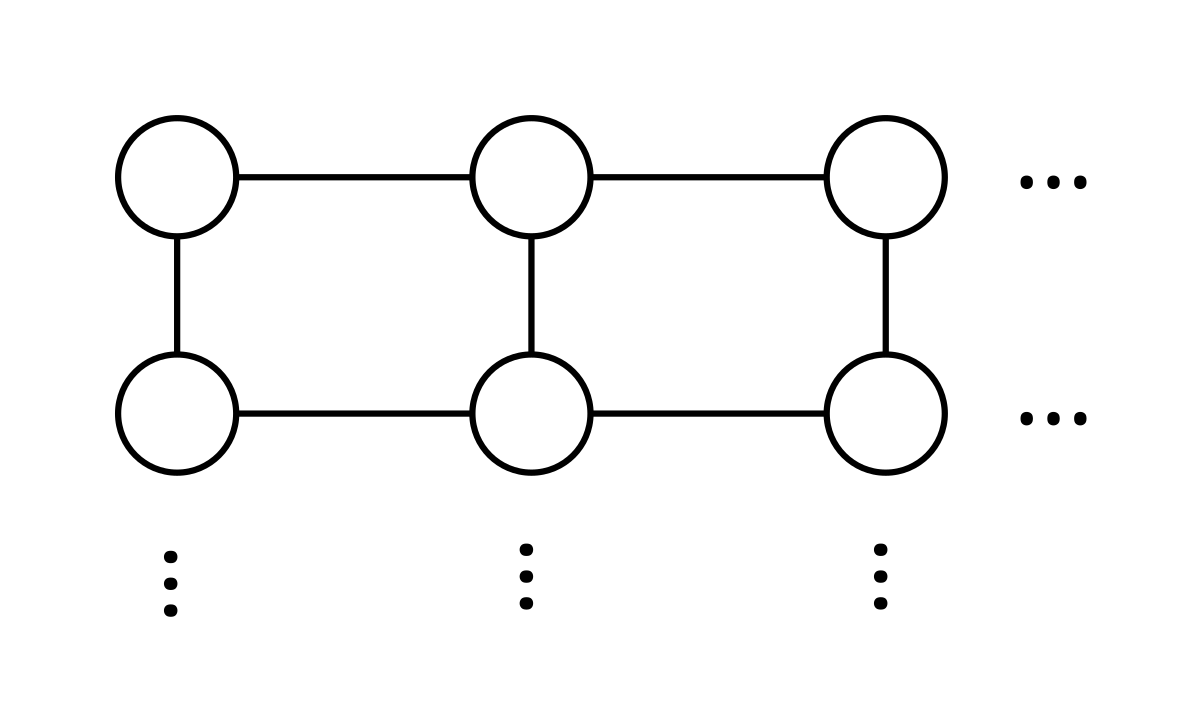
When building Hamiltonians with Quantum Solver, it is often required to create adjacency matrices that represent the lattice structure of the system under consideration, e.g., for the hopping term. Building those terms in 1d is relatively straight forward. For higher dimensions and more complicated lattices, however, this becomes more difficult. The HQS Lattice Builder and Lattice Validator are libraries that simplify this process and can directly be used with Quantum Solver.
As an example, we consider the computation of the groundstate of the tight-binding Hamiltonian, but this time on a rectangular lattice. The Hamiltonian is given by where is the set of all tuples such that is a neighbor of .
We start the example by specifying the required imports.
# NumPy, SciPy, and Matplotlib imports
import numpy as np
from scipy.sparse.linalg import eigsh
import matplotlib.pyplot as plt

# HQS Quantum Solver imports
from hqs_quantum_solver.spinless_fermions import (
    VectorSpace, Operator, lattice_term, annihilation
)

# HQS Lattice Builder/Validator imports
import lattice_builder
import lattice_validator
Then, we define the parameters of the simulation.
Mx = 5  # sites in x-direction
My = 4  # sitex in y-direction
N = 1  # particle count
t = 1  # hopping strengh
The next step is to create a Lattice Builder/Validator configuration
that specifies the Hamiltonian on an Mx My rectangular lattice.
In this example we have just one type of atom (lattice site) that is
repeated in the direction of the vectors in "lattice_vectors".
The hopping term is defined in the bonds variable, which adds an entry
of value -t into the hopping matrix for neighboring lattice sites.
For more details on the Lattice Builder configuration, take a look at the Hamiltonians in "Physics", HQS Lattice Documentation documentation, and at "Schema definitions", Lattice Validator Documentation.
system = {
    "site_type": "spinless_fermions",
    "cluster_size": [Mx, My, 1],
    "system_boundary_conditions": ["hard-wall", "hard-wall", "hard-wall"]
}
atoms = [{"id": 0}]
bonds = [
    {"id_from": 0, "id_to": 0, "translation": [1, 0, 0], "t": -t},
    {"id_from": 0, "id_to": 0, "translation": [0, 1, 0], "t": -t},
]
unitcell = {
    "atoms": atoms,
    "bonds": bonds,
    "lattice_vectors": [[1, 0, 0], [0, 1, 0]]
}
conf = {
    "system": system,
    "unitcell": unitcell
}
The configuration needs to be validated and normalized, which is done by using the Lattice Validator. Then, a Lattice Builder instance can be created. This instance is then passed to the lattice_term function, to convert it into an operator definition.
Note, if you do not need access to the Lattice Builder instance, you can also
directly pass the conf dict to lattice_term, which will take care of
the validation and builder construction.
is_valid, conf = lattice_validator.Validator().validateConfiguration(conf)
if not is_valid:
    raise ValueError(f"Configuration not valid: {conf}")
builder = lattice_builder.Builder(conf)

v = VectorSpace(sites=Mx * My, particle_numbers=N)
H = Operator(lattice_term(builder), domain=v)
After having obtained the Hamiltonian operator, the computation of the
groundstate and the definition of the site_occupation function are
the same as in the "Fermionic Basics" section.
k = min(12, H.shape[0] - 1)  # Number of eigenvalues to compute
evals, evecs = eigsh(H, k=k, which="SA")
groundstate = evecs[:, 0]

v_minus = v.copy(particle_number_change=-1)

def site_occupation(psi, j):
    annihilation_operator = Operator(annihilation(site=j), domain=v, codomain=v_minus)
    c_psi = annihilation_operator.dot(psi)
    return c_psi.conj() @ c_psi
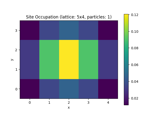
To plot the result we use the get_atom_positions method from the Lattice
Builder to show the groundstate occupation on a 2d grid.
occupations = np.zeros((My, Mx))
for j, position in enumerate(builder.get_atom_positions().tolist()):
    x, y = round(position[0]), round(position[1])
    # Set value for row=y and column=x.
    occupations[y, x] = site_occupation(groundstate, j)

plt.figure("site_occupation", clear=True)
plt.title(f"Site Occupation (lattice: {Mx}x{My}, particles: {N})")
plt.imshow(occupations, origin="lower", aspect="equal")
plt.xlabel("x")
plt.ylabel("y")
plt.xticks(np.arange(Mx))
plt.yticks(np.arange(My))
plt.colorbar()
plt.show()
Finally, we can run the code, to obtain a plot of the occupation, as shown below.
Complete Code
# Title    : HQS Quantum Solver using the Lattice Builder
# Filename : getting_started.py

# NumPy, SciPy, and Matplotlib imports
import numpy as np
from scipy.sparse.linalg import eigsh
import matplotlib.pyplot as plt

# HQS Quantum Solver imports
from hqs_quantum_solver.spinless_fermions import (
    VectorSpace, Operator, lattice_term, annihilation
)

# HQS Lattice Builder/Validator imports
import lattice_builder
import lattice_validator

# ===== Parameters =====

Mx = 5  # sites in x-direction
My = 4  # sitex in y-direction
N = 1  # particle count
t = 1  # hopping strengh

# ===== Definition of the Lattice =====

system = {
    "site_type": "spinless_fermions",
    "cluster_size": [Mx, My, 1],
    "system_boundary_conditions": ["hard-wall", "hard-wall", "hard-wall"]
}
atoms = [{"id": 0}]
bonds = [
    {"id_from": 0, "id_to": 0, "translation": [1, 0, 0], "t": -t},
    {"id_from": 0, "id_to": 0, "translation": [0, 1, 0], "t": -t},
]
unitcell = {
    "atoms": atoms,
    "bonds": bonds,
    "lattice_vectors": [[1, 0, 0], [0, 1, 0]]
}
conf = {
    "system": system,
    "unitcell": unitcell
}

# ===== Creation of the Hamiltonian =====

is_valid, conf = lattice_validator.Validator().validateConfiguration(conf)
if not is_valid:
    raise ValueError(f"Configuration not valid: {conf}")
builder = lattice_builder.Builder(conf)

v = VectorSpace(sites=Mx * My, particle_numbers=N)
H = Operator(lattice_term(builder), domain=v)

# ===== Computing the Eigenvalues and Eigenvectors =====

k = min(12, H.shape[0] - 1)  # Number of eigenvalues to compute
evals, evecs = eigsh(H, k=k, which="SA")
groundstate = evecs[:, 0]

# ===== Plotting the Site Occupations =====

v_minus = v.copy(particle_number_change=-1)

def site_occupation(psi, j):
    annihilation_operator = Operator(annihilation(site=j), domain=v, codomain=v_minus)
    c_psi = annihilation_operator.dot(psi)
    return c_psi.conj() @ c_psi

occupations = np.zeros((My, Mx))
for j, position in enumerate(builder.get_atom_positions().tolist()):
    x, y = round(position[0]), round(position[1])
    # Set value for row=y and column=x.
    occupations[y, x] = site_occupation(groundstate, j)

plt.figure("site_occupation", clear=True)
plt.title(f"Site Occupation (lattice: {Mx}x{My}, particles: {N})")
plt.imshow(occupations, origin="lower", aspect="equal")
plt.xlabel("x")
plt.ylabel("y")
plt.xticks(np.arange(Mx))
plt.yticks(np.arange(My))
plt.colorbar()
plt.show()