Introduction
HQS Quantum Solver gives you the ability to reduce the size of your quantum problem by letting you select the relevant subspaces. It will then provide you the relevant Hamiltonians and Operators. This documentation is geared towards spin systems, but the Quantum Solver can also address fermionic and bosonic problems. Note that a license for HQS Quantum Solver also includes a license for the HQS Electron Spectroscopy Database.
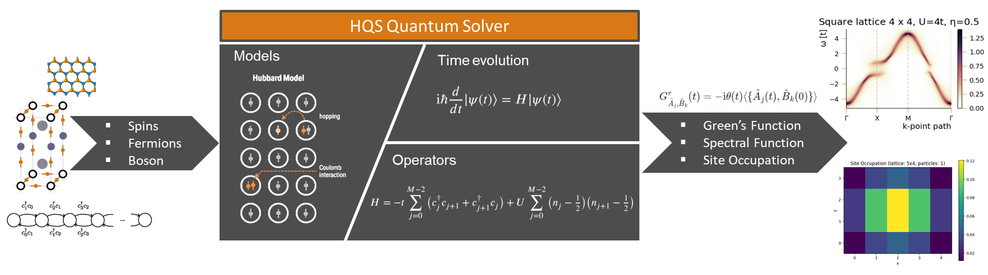
Providing a consistent and extensible interface, it offers routines for the construction of Hamiltonians and operators in either full configurational space or subspaces characterized by conserved quantities such as the spin or the particle number.
Applications
HQS Quantum Solver is a powerful tool for researchers and enthusiasts in the field of spin physics, quantum computing, and beyond. It can be used for a wide range of applications, including but not limited to:
-
Evaluating dynamic correlation functions for spin problems.
-
Calculate expectation values, static correlation functions, and eigenenergies.
-
Simulating coherent and incoherent time-evolution of spin.
-
For advanced users: studying interacting lattice models.
Getting started
HQS Quantum Solver is a tool that can be used in conjunction with other
HQStage modules by HQS Quantum Simulations GmbH. To install this module run
hqstage install hqs-quantum-solver
To use HQS Quantum Solver, you furthermore need to install the Intel Math Kernel Library (MKL), which can be done in three different ways.
-
You can use HQStage to install the MKL into the currently active virtual environment.
hqstage install mkl -
You can manually provide a version of the MKL by making sure that the file
libmkl_rt.sois found by the dynamic linker. That means, that a system-wide installation should be found automatically. -
You can install the MKL via pip.
pip install mkl
For a collection of examples to start using HQS Quantum Solver please refer to the Quick Start chapter.
Features
-
Enables exploitation of symmetries like spin conservation, particle number, or the fermion parity.
-
Flexible choice of combinations of subspaces, allows the choice of excitation subspaces adapted to your problem.
-
Calculation of static and dynamical correlations functions in frequency domain including the correction vector approach and the expansion in Chebyshev polynomials.
-
Krylov-based master equation solver, which is faster than QuTip in many regimes.
-
Extensibility: HQS Quantum Solver allows users to integrate their own backends, tools, and algorithms.
-
Interoperable: Integrates well with the scientific Python ecosystem, especially with NumPy and SciPy.
The API documentation can be found here.
Quantum Solver Concepts
In this chapter we discuss the elementary concepts needed to use HQS Quantum Solver.
Since quantum mechanical systems are described by linear operators, the first step in learning how to use Quantum Solver is how to construct and use operators. In Quantum Solver you define operators by specifying a vector space and an expression. The latter describes the mathematical terms that the operator is made of.
The examples in this chapter make use of the following imports.
from hqs_quantum_solver.spins import Operator, VectorSpace, spin_z, raising
Vector Spaces
All particle related modules, e.g., the
spins,
spinless_fermions, or
bosons module, contain a
VectorSpace class. Instantiating such a class is the first step in
constructing an operator in Quantum Solver.
In quantum mechanics, the states a system can be in determine the
vector space that the operator describing the system is defined on.
Therefore, VectorSpace objects are constructed by providing
parameters that describe these states, e.g., the
VectorSpace class from the
spins module is constructed by
providing the sites and the total_spin_z arguments.
The first argument defines the number of spins in the system,
while the second argument can be used to restrict to a sets of states with
a fixed total spin polarization.
We could, e.g., create a vector space object for a spin system with
four spins and the total spin polarization being restricted to zero
by the following code, where the total_spin_z spin quantum number is provided in units of .
VectorSpace(sites=4, total_spin_z=0)
A vector space object for a spin system with four spins and no restrictions on the total spin polarization could be constructed as follows.
VectorSpace(sites=4, total_spin_z="all")
Operator Expressions
The mathematical term that describes the operator is defined by an operator expression. The particle related modules, like the spins module, contain functions that return expression. Examples are the raising, magnetic_field_z, and isotropic_interaction functions. Expressions can be combined into arbitrary complex linear combinations, e.g.,
3 * spin_z(site=1) + 2 * spin_z(site=3)
corresponds to the term .
Many of these functions (also) take a coefficient array or vector as an input, e.g., the expression above could also be written as follows.
spin_z(coef=[0, 3, 0, 2])
Operators
To construct an operator, you need to create an instance of the desired operator class, which requires the operator expression and the vector space. We can construct the operator given by on a space where the total spin polarization is fixed to zero as follows.
v = VectorSpace(sites=4, total_spin_z=0)
H = Operator(3 * spin_z(site=1) + 2 * spin_z(site=3), domain=v)
Note that when the codomain attribute is not specified it is assumed
that the domain of the operator is equal to the codomain.
In cases, where the two spaces differ, the codomain attribute
must be explicitly given. This is the case, e.g., when applying the
spin raising operator on a space with a fixed total spin
polarization, as is done in the code below.
v = VectorSpace(sites=4, total_spin_z=0)
w = v.copy(total_spin_z_change=2)
A = Operator(raising(site=2), domain=v, codomain=w)
Once an operator object is constructed, it can be used by applying
methods like the
dot or
similar methods.
Furthremore, Quantum Solver operators are compatible to most
SciPy sparse routines and therefore can directly be used in functions
like eigsh.
Quick Start
This chapter contains Quick Start Guides, each of which is self-contained. Thus, the guides can be read in any order, and each guide is designed to get you started with a particular task as quickly as possible.
Spin-Flip Simulation
The Jupyter notebook corresponding to this section can be found here.
In this guide, you will learn how to load the Hamiltonian of a spin system, compute the energy levels of the Hamiltonian, and simulate the evolution of the corresponding system in time. We will use the Hamiltonian describing Acrylonitride () in a magnetic field, as you would encounter, e.g., in an NMR spectrometer.
First, we need to import the functions, classes and modules that are required for the script. Therefore, we create a Python script and add the following imports to our file, which we will explain, as we go along.
# Title    : HQS Quantum Solver Spin Flip Simulation
# Filename : spin_flip.py
from pathlib import Path

import numpy as np
import matplotlib.pyplot as plt
from scipy.sparse.linalg import eigsh

from struqture_py.spins import PauliHamiltonian

from hqs_quantum_solver.spins import (
    VectorSpace, Operator, lowering, struqture_term, spin_z, raising
)
from hqs_quantum_solver.evolution import evolve_krylov, observers
Next, we load the Hamiltonian description from a file in Struqture format. Struqture is a library providing an exchage format for quantum operators. (See the "Struqture" section for more information about using Struqture with Quantum Solver.) We have to store the file acrylonitride.json (right click, "Save As..."), which contains the description of the Hamiltonian, in the same directory as the Python script. Afterwards, we can load it as follows.
filepath = Path("acrylonitride.json")
hamiltonian_info = PauliHamiltonian().from_json(filepath.read_text())
So far, we have only loaded a description of a Hamiltonian. To use it,
we need to turn it into an actual Operator that, e.g., can be applied
to a state vector. In addition to the definition of the operator,
Quantum Solver needs the vector space that the operator is defined on.
Since we are dealing with a spin system, we create a
VectorSpace object from the
spins module.
Vector spaces, as used in quantum mechanics, are defined by the states
they represent. The states of the system are defined by the
sites and the total_spin_z arguments. The former sets the number of
spins in the system, and the latter can be used to only include states
with a given total spin polarization. Since we want to include all
states, we set total_spin_z to "all".
v = VectorSpace(sites=hamiltonian_info.current_number_spins(), total_spin_z="all")
Having constructed the vector space, we can now create the Hamiltonian as an instance of type Operator.
hamiltonian = Operator(struqture_term(hamiltonian_info), domain=v, dtype=complex)
Herein, we used the struqture_term
function to tell Quantum Solver that the input is in Struqture format.
Furthermore, we enforced the construction of a complex-valued operator
by setting dtype to complex. (Setting dtype is optional,
but since we want to compute a time evolution of the system, which requires
complex state vectors, having a complex operator yields better performance.)
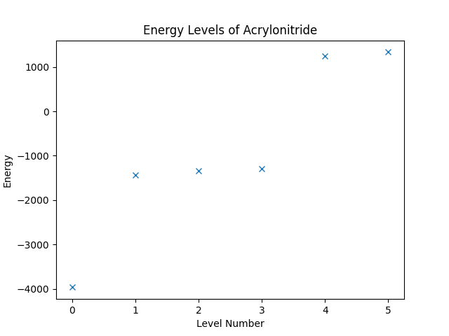
We can now obtain the energy levels of the system by computing the eigenvalues of the operator. The Operator class is compatible to SciPy, such that we can directly call the eigsh on the operator, and then use Matplotlib to plot the result. (Note that the eigsh function does not return the eigenvalues in a sorted order when the operator is complex.)
eigvals, eigvecs = eigsh(hamiltonian, k=6, which="SA")
sorted_indices = np.argsort(eigvals)

plt.figure("energy-levels")
plt.title("Energy Levels of Acrylonitride")
plt.xlabel("Level Number")
plt.ylabel("Energy")
plt.plot(eigvals[sorted_indices], "x")
Running the script up to this point should result in an image as shown below.
We shall now turn to the simulation of the time evolution of the system described by the Hamiltonian. The first thing that we need is to setup the initial wave function of the system. For that, we want to take the groundstate of the system and flip one of the spins. Flipping the th spin is done by applying the operator , which needs to be built first.
Quantum Solver has a selection of high-level functions that can be used to describe operators. For our purpose we use the raising and lowering functions, which describe the and operator, respectively. Since Quantum Solver allows for building of arbitrary linear combinations of those operator descriptions, we can build the desired spin-flip operator for the site with index 2 as follows.
flip = Operator(raising(site=2) + lowering(site=2), domain=v, dtype=complex)
The spin-flip operator can be applied to a wave function by using the .dot
method of the operator.
groundstate = eigvecs[:, sorted_indices[0]]
initial_wavefunction = flip.dot(groundstate)
Since inspecting the wave function directly is usually not very insightful, we need to perform an additional step, before we run a time simulation. We want to look at the expectation value of observables, in this case the spin polarizations for all sites of the system. The operator is described by the spin_z function, and we can create a list of all desired observables in the following way.
observables = [
    Operator(spin_z(site=j), domain=v, dtype=complex) for j in range(v.sites)
]
With the observables at hand, we can now create an list containing the time values at which we want to evaluate the wave function, call the evolve_krylov function to perform the simulation, and then stack the list of observations into a single NumPy array.
ts = np.linspace(0, 1e-1, 100)
result = evolve_krylov(
    hamiltonian, initial_wavefunction, ts,
    observer=observers.expectation(observables)
)
observations = np.stack(result.observations)
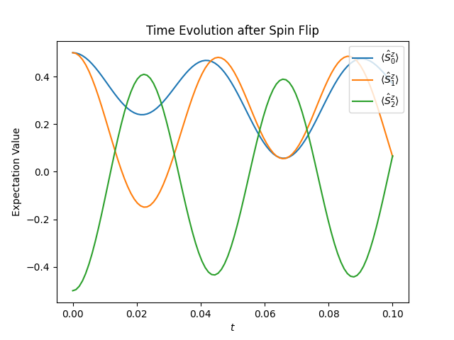
The result can then be visualized using the code below.
plt.figure("time-evolution")
plt.title("Time Evolution after Spin Flip")
plt.xlabel("$t$")
plt.ylabel("Expectation Value")
for j in range(observations.shape[1]):
    plt.plot(ts, observations[:, j], label=f"$\\langle \\hat{{S}}^z_{j} \\rangle$")
plt.legend(loc="upper right")
plt.show()
The figure below shows the resulting plot, which shows how the spins polarization oscillates after the spin flip.
Complete Code
# Title    : HQS Quantum Solver Spin Flip Simulation
# Filename : spin_flip.py
from pathlib import Path

import numpy as np
import matplotlib.pyplot as plt
from scipy.sparse.linalg import eigsh

from struqture_py.spins import PauliHamiltonian

from hqs_quantum_solver.spins import (
    VectorSpace, Operator, lowering, struqture_term, spin_z, raising
)
from hqs_quantum_solver.evolution import evolve_krylov, observers

# ===== Loading and Building the Hamiltonian =====

filepath = Path("acrylonitride.json")
hamiltonian_info = PauliHamiltonian().from_json(filepath.read_text())

v = VectorSpace(sites=hamiltonian_info.current_number_spins(), total_spin_z="all")
hamiltonian = Operator(struqture_term(hamiltonian_info), domain=v, dtype=complex)

# ===== Energy Levels =====

eigvals, eigvecs = eigsh(hamiltonian, k=6, which="SA")
sorted_indices = np.argsort(eigvals)

plt.figure("energy-levels")
plt.title("Energy Levels of Acrylonitride")
plt.xlabel("Level Number")
plt.ylabel("Energy")
plt.plot(eigvals[sorted_indices], "x")

# ===== Spin Flip =====

flip = Operator(raising(site=2) + lowering(site=2), domain=v, dtype=complex)

groundstate = eigvecs[:, sorted_indices[0]]
initial_wavefunction = flip.dot(groundstate)

# ===== Time Evolution =====

observables = [
    Operator(spin_z(site=j), domain=v, dtype=complex) for j in range(v.sites)
]

ts = np.linspace(0, 1e-1, 100)
result = evolve_krylov(
    hamiltonian, initial_wavefunction, ts,
    observer=observers.expectation(observables)
)
observations = np.stack(result.observations)

plt.figure("time-evolution")
plt.title("Time Evolution after Spin Flip")
plt.xlabel("$t$")
plt.ylabel("Expectation Value")
for j in range(observations.shape[1]):
    plt.plot(ts, observations[:, j], label=f"$\\langle \\hat{{S}}^z_{j} \\rangle$")
plt.legend(loc="upper right")
plt.show()
Lindblad Simulation
The Jupyter notebook corresponding to this section can be found here.
In this guide you will learn how to create a simulation of the Lindblad equation, which is given by where is the Lindbladian with Here, is a Hamiltonian of a spin system. For this guide, we choose the Hamiltonian of the Heisenberg spin chain, i.e.,
Imports and Parameters
Throughout this guide, we will make use of the following imports.
import matplotlib.pyplot as plt
import numpy as np
import numpy.random
from matplotlib import animation
from scipy.linalg import toeplitz

from hqs_quantum_solver.spins import (
    VectorSpace, Operator, SpinState, isotropic_interaction)
from hqs_quantum_solver.util import unit_vector
from hqs_quantum_solver.lindblad import Lindbladian
from hqs_quantum_solver.evolution import evolve_krylov, observers
Furthermore, we make use of the parameters as shown below.
n_spins = 6  # The number of spins.
t_end = 10   # The duration of the simulation.
J = 1        # The interaction strength.
Hamiltonian and Lindblad
To construct the Lindbladian, we first have to define the vector space that we are using, then construct the Hamiltonian, and then combine the two to obtain the Lindblad operator. We start with the vector space.
The vector space is defined by creating a
VectorSpace object from the
spins module.
The vector spaces we use in quantum mechanics are defined by the
states they represent. Thus, to construct the
VectorSpace object, we have to describe
the states of the system. First, we give the sites argument to
specify the number of spins in the system. Second, we give the
total_spin_z argument, which can be used to only include the states with
a given total spin polarization. Since we do not want to restrict the
total spin, we provide "all" as an argument.
v = VectorSpace(sites=n_spins, total_spin_z="all")
To construct a spin operator in HQS Quantum Solver, we need to pass an expression that describes the operator to the constructor of the Operator class. We use the isotropic_interaction function to obtain the desired expression. This function takes a matrix, where the entry at index determines the interaction strength of site to site and vice versa. By providing a matrix where the first upper off-diagonal is set to a constant value and the remaining entries set to zero, we obtain the desired spin chain model.
coef = J * toeplitz(np.zeros(v.sites), unit_vector(v.sites, 1))
H = Operator(isotropic_interaction(coef), domain=v, dtype=complex)
Next, we need to set up the coefficient matrices , , and . For this example, we choose these matrices as random, positive definite matrices. Once the matrices are constructed, we pass them together with the Hamiltonian to the constructor of the Lindbladian class, giving us the desired Lindblad operator.
rng = numpy.random.default_rng(1234)

def random_positive_definite(low, high, shape):
    r = rng.uniform(low, high, shape)
    return r.T.conj() @ r

gamma_z = random_positive_definite(0, 0.3, (v.sites, v.sites))
gamma_p = random_positive_definite(0, 0.2, (v.sites, v.sites))
gamma_m = random_positive_definite(0, 0.1, (v.sites, v.sites))

L = Lindbladian(H, gamma_z, gamma_p, gamma_m)
Initial State
Before we can simulate the time evolution, we need to define the
initial state of the simulation. We choose
where
.
The vector is constructed by calling the
fock_state function with
a list containing SpinState.UP followed by multiple SpinState.DOWN
entries.
state = v.fock_state([SpinState.UP] + [SpinState.DOWN] * (n_spins-1))
rho = state[:,np.newaxis] @ state[:,np.newaxis].T.conj()
Time Evolution
We can finally perform the actual time evolution of the system.
The form of the Lindblad equation listed at the beginning is compatible
with the regular time-stepping functions provided by Quantum Solver.
Here, we want to use the
evolve_krylov function.
We provide the operator, the initial state, and a list of time points at
which to evaluate the state of the system. Note, that internally a
step-size is chosen that guarantees the desired accuracy. The time points
are only used for the evaluation.
Furthermore, by passing observer=observers.state() we instruct the method to
record the full state at each time point. Finally, we provide a
progress callback that displays the current state of the simulation
while the simulation is in progress.
timesteps = np.linspace(0, t_end)

def progress(t):
    print(f"t = {t:7.2f}", end="\r", flush=True)

result = evolve_krylov(
    L, rho, timesteps, observer=observers.state(), progress=progress)

print()
The state of the system for each time point in timesteps is now
stored in result.observations as a list. We can use Matplotlib to
create an animation.
fig, ax = plt.subplots()
image = ax.imshow(np.abs(result.observations[0]), cmap='magma_r', vmin=0, vmax=1)
plt.colorbar(image)

def update(frame):
    ax.set_title(f'State density at $t = {timesteps[frame]:.2f}$')
    image.set_data(np.abs(result.observations[frame]))
    return [image]

ani = animation.FuncAnimation(fig, update, frames=len(result.observations))
plt.show()
Running the script should produce the following animation.
Complete Code
# Title    : HQS Quantum Solver Linblad Solver
# Filename : lindblad.py

# ===== Imports =====

import matplotlib.pyplot as plt
import numpy as np
import numpy.random
from matplotlib import animation
from scipy.linalg import toeplitz

from hqs_quantum_solver.spins import (
    VectorSpace, Operator, SpinState, isotropic_interaction)
from hqs_quantum_solver.util import unit_vector
from hqs_quantum_solver.lindblad import Lindbladian
from hqs_quantum_solver.evolution import evolve_krylov, observers

# ===== Parameters =====

n_spins = 6  # The number of spins.
t_end = 10   # The duration of the simulation.
J = 1        # The interaction strength.

# ===== Constructing the Lindbladian =====

v = VectorSpace(sites=n_spins, total_spin_z="all")

coef = J * toeplitz(np.zeros(v.sites), unit_vector(v.sites, 1))
H = Operator(isotropic_interaction(coef), domain=v, dtype=complex)

rng = numpy.random.default_rng(1234)

def random_positive_definite(low, high, shape):
    r = rng.uniform(low, high, shape)
    return r.T.conj() @ r

gamma_z = random_positive_definite(0, 0.3, (v.sites, v.sites))
gamma_p = random_positive_definite(0, 0.2, (v.sites, v.sites))
gamma_m = random_positive_definite(0, 0.1, (v.sites, v.sites))

L = Lindbladian(H, gamma_z, gamma_p, gamma_m)

# ===== Initial State =====

state = v.fock_state([SpinState.UP] + [SpinState.DOWN] * (n_spins-1))
rho = state[:,np.newaxis] @ state[:,np.newaxis].T.conj()

# ===== Time Evolution =====

timesteps = np.linspace(0, t_end)

def progress(t):
    print(f"t = {t:7.2f}", end="\r", flush=True)

result = evolve_krylov(
    L, rho, timesteps, observer=observers.state(), progress=progress)

print()

# ===== Visualization =====

fig, ax = plt.subplots()
image = ax.imshow(np.abs(result.observations[0]), cmap='magma_r', vmin=0, vmax=1)
plt.colorbar(image)

def update(frame):
    ax.set_title(f'State density at $t = {timesteps[frame]:.2f}$')
    image.set_data(np.abs(result.observations[frame]))
    return [image]

ani = animation.FuncAnimation(fig, update, frames=len(result.observations))
plt.show()
Combining Vector Spaces
The Jupyter notebook corresponding to this section can be found here.
In this guide you will learn how to run simulations with a large number of spins by computing on a subspace given by a restricted set of states. To demonstrate this approach, we consider the following spin system. We split the sites into sites that experience a strong interaction and sites that experience a weak interaction, while a magnetic field is acting on all sites. More precisely, we consider the Hamiltonian
where and . Furthermore, we choose the entries in the strictly upper triangle of to be uniformly randomly distributed between and and the remaining entries to be zero.
The Hamiltonian is defined on the space , where contains all possible spin states on the first sites and contains the states where at most one spin of the remaining sites is in the state. While the number of states represented by grows exponentially with , the number of states represented by only grows linearly with . Thus, we can perform computations with large values for .
Imports and Parameters
Throughout this guide, we will make use of the following imports.
import numpy as np
from scipy.sparse.linalg import eigsh
import matplotlib.pyplot as plt

from hqs_quantum_solver.spins import (
    VectorSpace, Operator, magnetic_field_z, isotropic_interaction, spin_z)
Furthermore, we use the following parameters.
sites_part1 = 12  # Number of sites of the first part
sites_part2 = 50  # Number of sites of the second part

B = -1.5      # The magnetic field strength
J_strong = 1  # The strength of the strong interaction
J_weak = 0.2  # The strength of the weak interaction
Vector Spaces
We want to construct the Hamiltonian of the system, which requires to define the vector space that the operator is defined on, first.
We start by defining the space , which we do by constructing a
VectorSpace object from the
spins module. The vector space object is
defined by the states that it represents, which are in turn defined by
the number of spins in the system (sites) and the restriction on the
total spin polarization in -direction (total_spin_z).
Since we do not want to restrict the total spin polarization, we just
pass "all" for this argument.
v1 = VectorSpace(sites=sites_part1, total_spin_z="all")
To create the space , we need to combine two spaces. The first space just
represents the state where all spins are in the state, and the
second space represents the states where just one spin is in the
state. The first one is characterized by a total spin polarization of
and the second one by a total spin polarization of
.
We want a vector space that represents the states represented by both
spaces combined. Using the |
(or the span method)
the desired space is constructed from the individual spaces. Note that
the total spin is specified in units of .
v2 = (VectorSpace(sites=sites_part2, total_spin_z=-sites_part2)
      | VectorSpace(sites=sites_part2, total_spin_z=-sites_part2 + 2))
Finally, we can use the * operator to compute the desired tensor product
.
v = v1 * v2
The next step is to define the coefficient matrices.
Building Operators
Building an operator in Quantum Solver works by calling the constructor of the desired Operator class with an expression describing the operator and the vector space.
The expression describing the magnetic field can be obtained by using
the magnetic_field_z function.
By providing the coef argument, we can specify the magnetic field in
-direction per site as a vector. This vector is constructed by the
code below.
B_coef = np.full(v.sites, B)
To define the interaction part of the Hamiltonian, we want to use the isotropic_interaction function, which gives the desired expression when given an appropriate coefficient matrix. Looking at the documentation of the function shows that we can describe the term by providing a matrix where the first entries of the first upper off-diagonal are set to and the remaining entries set to zero. This matrix is constructed as follows.
d1 = np.where(np.arange(v.sites - 1) < v1.sites - 1, 1, 0)
J_strong_mat = J_strong * np.diag(d1, 1)
The second term is represented by a coefficient matrix with random coefficients in .
rng = np.random.default_rng(314159)

J_weak_mat = J_weak * np.triu(rng.uniform(0, 1, (v.sites, v.sites)), 1)
Now, that we have the coefficient matrices, we can build the Hamiltonian.
The interaction term, however, maps onto states that are not part of
the vector space . Oftentimes, this is an indicator for an error. Hence, we
have to pass strict=False as an argument to the Operator constructor, to
explicitly allow Quantum Solver to drop states not present in the vector
space.
H = Operator(
    magnetic_field_z(coef=B_coef) + isotropic_interaction(J_strong_mat + J_weak_mat),
    domain=v,
    strict=False
)
Spectrum & Eigenvectors
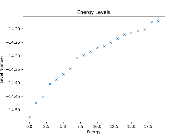
Having constructed the Hamiltonian, we can now use it to, e.g., compute the energy levels of the system. Since Quantum Solver operators are compatible with SciPy, we can directly use the eigsh function from SciPy to compute the eigenvalues.
eigvals, eigvecs = eigsh(H, k=20, which='SA')
The eigenvalues are the energy levels of the system and can be plotted as follows, while the resulting figure is shown below.
plt.figure()
plt.title('Energy Levels')
plt.xlabel('Level Number')
plt.ylabel('Energy')
plt.plot(eigvals, 'x')
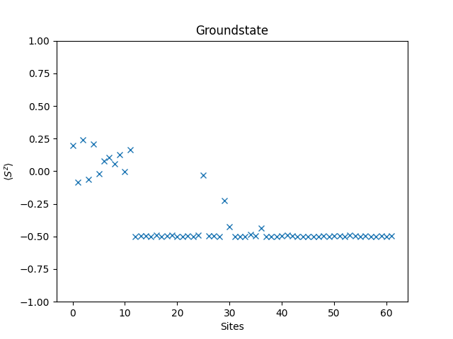
Another interesting quantity to look at is the expectation value of the spin polarization of the groundstate, i.e., for . The operator is provided by the spin_z function, and the application of the operator by the dot method, so the implementation is straight forward.
observables = [Operator(spin_z(site=j), domain=v) for j in range(v.sites)]

def spin_z_expectation(psi):
    return [np.vecdot(psi, o.dot(psi)) for o in observables]
The result can be plotted using the following code, and the resulting figure is shown below.
groundstate = eigvecs[:,0]

plt.figure()
plt.title('Groundstate')
plt.xlabel('Sites')
plt.ylabel(r'$\langle S^z \rangle$')
plt.ylim(-1, 1)
plt.plot(spin_z_expectation(groundstate), 'x')

plt.show()
Complete Code
# Title    : HQS Quantum Solver Combining Vector Spaces
# Filename : combining-spaces.py

# ===== Imports =====

import numpy as np
from scipy.sparse.linalg import eigsh
import matplotlib.pyplot as plt

from hqs_quantum_solver.spins import (
    VectorSpace, Operator, magnetic_field_z, isotropic_interaction, spin_z)

# ===== Parameters =====

sites_part1 = 12  # Number of sites of the first part
sites_part2 = 50  # Number of sites of the second part

B = -1.5      # The magnetic field strength
J_strong = 1  # The strength of the strong interaction
J_weak = 0.2  # The strength of the weak interaction

# ===== Vector Spaces =====

v1 = VectorSpace(sites=sites_part1, total_spin_z="all")

v2 = (VectorSpace(sites=sites_part2, total_spin_z=-sites_part2)
      | VectorSpace(sites=sites_part2, total_spin_z=-sites_part2 + 2))

v = v1 * v2

# ===== Building the Hamiltonian =====

B_coef = np.full(v.sites, B)

d1 = np.where(np.arange(v.sites - 1) < v1.sites - 1, 1, 0)
J_strong_mat = J_strong * np.diag(d1, 1)

rng = np.random.default_rng(314159)

J_weak_mat = J_weak * np.triu(rng.uniform(0, 1, (v.sites, v.sites)), 1)

H = Operator(
    magnetic_field_z(coef=B_coef) + isotropic_interaction(J_strong_mat + J_weak_mat),
    domain=v,
    strict=False
)

# ===== Plotting the Energy Levels =====

eigvals, eigvecs = eigsh(H, k=20, which='SA')

plt.figure()
plt.title('Energy Levels')
plt.xlabel('Level Number')
plt.ylabel('Energy')
plt.plot(eigvals, 'x')

# ===== Plotting the Spin Polarization =====

observables = [Operator(spin_z(site=j), domain=v) for j in range(v.sites)]

def spin_z_expectation(psi):
    return [np.vecdot(psi, o.dot(psi)) for o in observables]

groundstate = eigvecs[:,0]

plt.figure()
plt.title('Groundstate')
plt.xlabel('Sites')
plt.ylabel(r'$\langle S^z \rangle$')
plt.ylim(-1, 1)
plt.plot(spin_z_expectation(groundstate), 'x')

plt.show()
Struqture Hamiltonians
The Jupyter notebook corresponding to this section can be found here.
In this guide you will learn how to create operators using Struqture, which is a library that is used to describe quantum mechanical operators and systems. It can be used as an input to HQS Quantum Solver for defining spin systems.
For this chapter, we use the system of antiferromagnetically coupled spins defined by the Hamiltonian , where
as an example.
Imports & Parameters
Throughout this chapter, we will use the following imports.
import numpy as np
import matplotlib.pyplot as plt
from scipy.sparse.linalg import eigsh

from struqture_py import PauliHamiltonian

from hqs_quantum_solver.spins import (
    VectorSpace, Operator, magnetic_field_z, struqture_term
)
Furthermore, we will make use of the following parameters.
M = 8    # number of sites/spins
J = 1.0  # interaction strength
B = 3.0  # magnetic field strength (will be introduced later)
Building Operators
Hamiltonians for spin systems can be described in Struqture using the PauliHamiltonian class. (Other options for describing spin systems are the PauliOperator and PlusMinusOperator classes.) The class describes a sum of products of operators. Each operator acts on a specific site of the system, and each product has at most one operator per site. More precisely, the operators have the form Inhere, , , and . The previously defined Hamiltonian can be written in this form: we have that which has the desired shape.
To define the Hamiltonian using Struqture, we first create an object of type
PauliHamiltonian and then add the individual products using the
.add_operator_product method.
Each product is given by a string, describing the operator product, and the
corresponding coefficient.
The string consecutively lists the terms of the product,
where each factor is represented by a number followed by a character.
The number defines the site the operator is acting on, and the character
defines the type of the operator, e.g. "2X3X" describes the product
.
In the following code, we use
Python format strings
to build the required strings.
interaction = PauliHamiltonian()

for j in range(M - 1):
    interaction.add_operator_product(f"{j}X{j+1}X", 0.25 * J)
    interaction.add_operator_product(f"{j}Y{j+1}Y", 0.25 * J)
    interaction.add_operator_product(f"{j}Z{j+1}Z", 0.25 * J)

print(interaction)
Running the code above creates the desired operator and prints the following output, which shows how Struqture stores the operator, where each line gives one summand from the formula for the Hamiltonian.
PauliHamiltonian{
0X1X: 5e-1,
0Y1Y: 5e-1,
0Z1Z: 5e-1,
1X2X: 5e-1,
1Y2Y: 5e-1,
1Z2Z: 5e-1,
2X3X: 5e-1,
2Y3Y: 5e-1,
2Z3Z: 5e-1,
3X4X: 5e-1,
3Y4Y: 5e-1,
3Z4Z: 5e-1,
4X5X: 5e-1,
4Y5Y: 5e-1,
4Z5Z: 5e-1,
5X6X: 5e-1,
5Y6Y: 5e-1,
5Z6Z: 5e-1,
}
Having a description of the Hamiltonian, we can create an actual operator
that we can use in computations. The first thing to do is to convert the
Struqture object into a Quantum Solver expression, using the
struqture_term function.
Then, we need to create a VectorSpace
object that described the vector space the operator is acting on, and
finally an
Operator
object, by passing in the expression describing the operator and the vector
space. Note that we can use the .current_number_spins method to set
the number of sites in the vector space.
v = VectorSpace(sites=interaction.current_number_spins(), total_spin_z="all")
hamiltonian = Operator(struqture_term(interaction), domain=v)
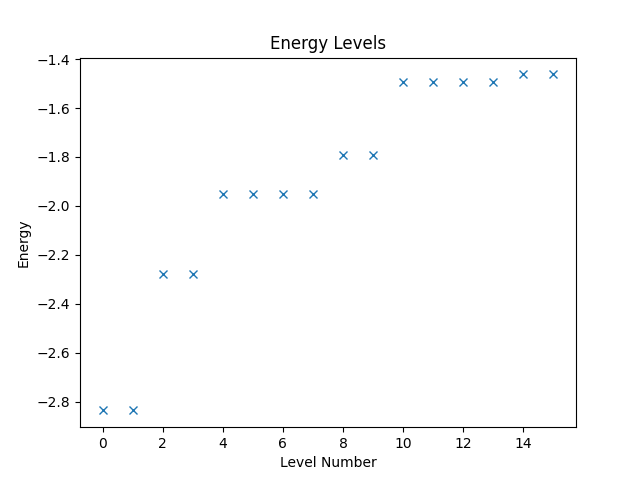
With the operator, we can now compute and plot the energy levels. Since Quantum Solver operators are compatible to SciPy, we can directly call the eigsh function from SciPy to obtain the energy levels. Then we use Matplotlib to create a plot of the levels.
eigvals, eigvecs = eigsh(hamiltonian, k=16, which="SA")

plt.figure("energy")
plt.title("Energy Levels")
plt.xlabel("Level Number")
plt.ylabel("Energy")
plt.plot(eigvals, "x")
The resulting figure is shown below.
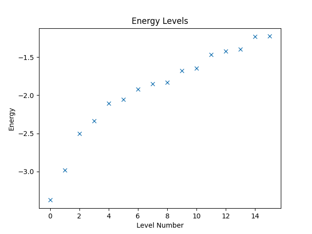
Restricting the Spin Polarization
If we know that we only need to consider states with a given total spin polarization in direction, e.g., when considering Hamiltonians that conserve the total spin polarization, we can restrict the states the vector space represents accordingly. This restriction can significantly reduce the amount of computational work needed. Say, we know that the total spin polarization is zero. Then, we can create the restricted vector space and the operator that is defined on it as follows.
w = VectorSpace(sites=interaction.current_number_spins(), total_spin_z=0)
hamiltonian2 = Operator(struqture_term(interaction), domain=w)
Computing and plotting the energy levels can then be done as before.
eigvals2, eigvecs2 = eigsh(hamiltonian2, k=16, which="SA")

plt.figure("energy-restricted")
plt.title("Energy Levels")
plt.xlabel("Level Number")
plt.ylabel("Energy")
plt.plot(eigvals2, "x")
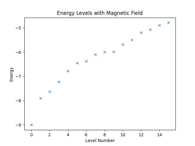
Combining Expressions
Next, we want to consider a slightly more complicated example. Assume that the spin system that we have defined at the beginning of this chapter is exposed to a magnetic field in direction of the -axis. More precisely, we want to consider the Hamiltonian that is given by
If we wanted, we could build the entire Hamiltonian using Struqture. There is, however, an easier way. Quantum Solver has already a definition of the magnetic-field term, namely the magnetic_field_z function. Furthermore, Quantum Solver allows building of arbitrary linear combination of Quantum Solver expressions. Hence, we can combine the Struqture definition of the spin interaction with the magnetic_field_z function, which is shown below.
hamiltonian3 = Operator(
    magnetic_field_z(coef=B * np.ones(v.sites)) + struqture_term(interaction),
    domain=w
)
Then, again, we can compute the energy levels and plot them.
eigvals3, eigvecs3 = eigsh(hamiltonian3, k=16, which="SA")

plt.figure("energy-with-field")
plt.title("Energy Levels with Magnetic Field")
plt.xlabel("Level Number")
plt.ylabel("Energy")
plt.plot(eigvals3, "x")

plt.show()
Finally, running the code produces the figure below.
Complete Code
# Title    : Using Struqture with HQS Quantum Solver
# Filename : struqture.py

# ===== Imports and Parameters =====

import numpy as np
import matplotlib.pyplot as plt
from scipy.sparse.linalg import eigsh

from struqture_py import PauliHamiltonian

from hqs_quantum_solver.spins import (
    VectorSpace, Operator, magnetic_field_z, struqture_term
)

M = 8    # number of sites/spins
J = 1.0  # interaction strength
B = 3.0  # magnetic field strength (will be introduced later)

# ===== Struqture Definition of the System =====

interaction = PauliHamiltonian()

for j in range(M - 1):
    interaction.add_operator_product(f"{j}X{j+1}X", 0.25 * J)
    interaction.add_operator_product(f"{j}Y{j+1}Y", 0.25 * J)
    interaction.add_operator_product(f"{j}Z{j+1}Z", 0.25 * J)

print(interaction)

# ===== Creating the Operator =====

v = VectorSpace(sites=interaction.current_number_spins(), total_spin_z="all")
hamiltonian = Operator(struqture_term(interaction), domain=v)

eigvals, eigvecs = eigsh(hamiltonian, k=16, which="SA")

plt.figure("energy")
plt.title("Energy Levels")
plt.xlabel("Level Number")
plt.ylabel("Energy")
plt.plot(eigvals, "x")

# ===== Restricted Sz =====

w = VectorSpace(sites=interaction.current_number_spins(), total_spin_z=0)
hamiltonian2 = Operator(struqture_term(interaction), domain=w)

eigvals2, eigvecs2 = eigsh(hamiltonian2, k=16, which="SA")

plt.figure("energy-restricted")
plt.title("Energy Levels")
plt.xlabel("Level Number")
plt.ylabel("Energy")
plt.plot(eigvals2, "x")

# ===== Combining Expressions =====

hamiltonian3 = Operator(
    magnetic_field_z(coef=B * np.ones(v.sites)) + struqture_term(interaction),
    domain=w
)

eigvals3, eigvecs3 = eigsh(hamiltonian3, k=16, which="SA")

plt.figure("energy-with-field")
plt.title("Energy Levels with Magnetic Field")
plt.xlabel("Level Number")
plt.ylabel("Energy")
plt.plot(eigvals3, "x")

plt.show()
Introduction to Electron Spectroscopy
The Jupyter notebooks corresponding to this section can be found here.
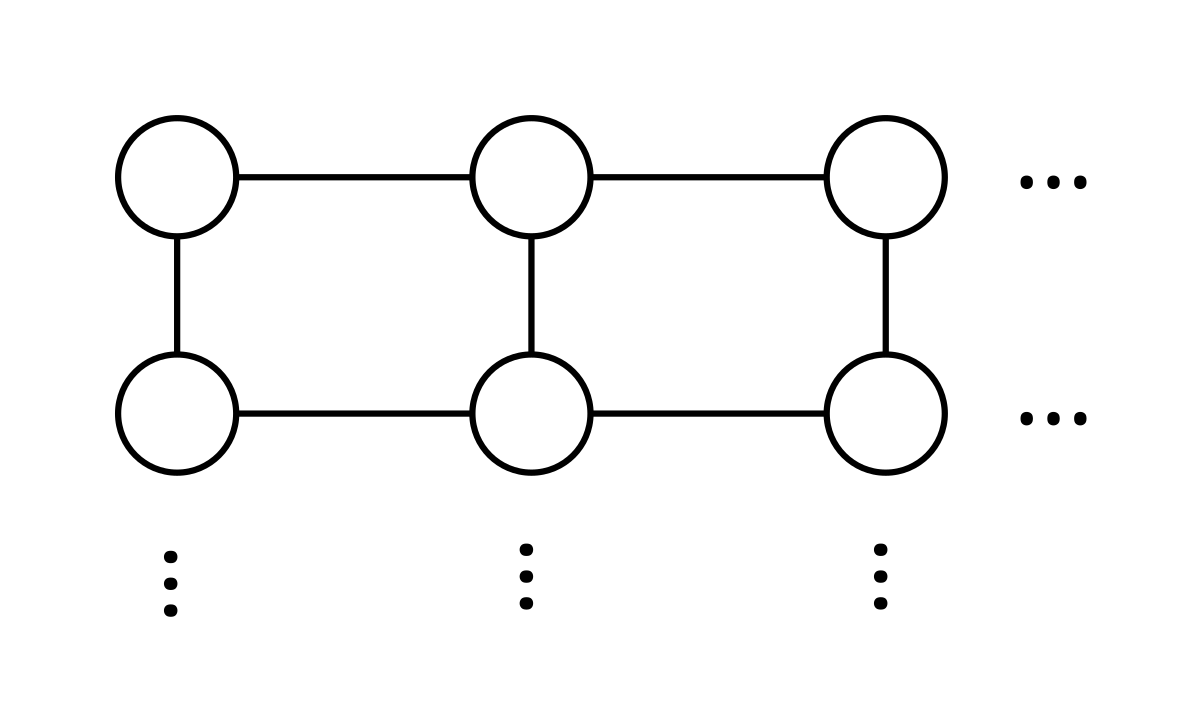
In this chapter, we calculate splittings, , of molecules using HQS Quantum Solver. The value is the difference between the lowest singlet and the triplet electronic states of a molecule. The corresponding database contains specialized Hamiltonians for three molecules: furane, thiophene and cyclopentadiene, derived via random phase approximation (RPA). This method involves partitioning the system into an active space that interacts with the environment. The active subspace consists of two orbitals that interact with a bath made up of other molecular orbitals:
NOTES:
- The Hamiltonian is derived in terms of qubits. The number of them can be varied and serves as an input parameter.
- One can return the full Hamiltonian or the truncated one, where number of qubits defines the truncation: the less qubits are available, the higher the truncation level.
- Hamiltonians are generated in the HQS Struqture format.
- The database also contains molecular structure and reference value of singlet-triplet splittings computed with quantum chemistry methods.

Imports & Parameters
To use HQS Quantum Solver and Struqture import the following:
from hqs_quantum_solver.spins import VectorSpace, Operator
from hqs_quantum_solver.spins import struqture_term
from electron_spectroscopy import Hamiltonians
from struqture_py.spins import PauliHamiltonian
Additionally import the following general-purpose libraries:
import numpy as np
import scipy.sparse as sparse
import matplotlib.pyplot as plt
from scipy.sparse.linalg import eigsh
Next, we need to import the electron_spectroscopy database and obtain one of the Hamiltonians:
from electron_spectroscopy import Hamiltonians

H = Hamiltonians.stored_hamiltonians["cyclopentadiene"]
Each Hamiltonian is a Python class containing numerical parameters.
Full Hamiltonians are currently computationally intractable, therefore, one should create a truncated one, restricted in number of qubits used for the environment. To create a truncated Hamiltonian in the struqture format run:
trunc_H = H.truncate_env(n_qubits=4, allow_large=False)
The maximum number of qubits to be solved by HQS Quantum Solver is 62. To generate more, one should set allow_large=True. The maximum number of qubits is equal to the length of the H.omega array and depends on the molecule. (In all examples this value is of the order of thousands.)
Alternatively, one may directly read-in a previously generated truncated Struqture Hamiltonian saved as a .json-file:
ham_json = "cyclopentadiene_4_qubits.json"
with open(ham_json, "r", encoding="utf-8") as f:
  trunk_H = PauliHamiltonian.from_json(f.read())
Reference Data
If you are interested in the molecular systems you are studying you can inspect the molecular geometries:
from electron_spectroscopy.xyzfiles import stored_structures

print(stored_structures["cyclopentadiene"])
To get a quantum chemistry reference value of singlet-triplet splitting and the information on the calculation run:
from electron_spectroscopy.data_dict import excitation_energies

print(excitation_energies["cyclopentadiene"])
Building Hamiltonian in HQS Quantum Solver
We first define the vector space for the system of two orbitals:
num_spins_cas = 2
v_cas = VectorSpace(sites=num_spins_cas, total_spin_z="all")
Then we create vector spaces for the bosonic bath for empty, single and double excitations in the bath:
v_bath_0 = VectorSpace(sites =num_spins_bath, total_spin_z=-num_spins_bath)
v_bath_1 = VectorSpace(sites=num_spins_bath, total_spin_z=-num_spins_bath + 2)
v_bath_2 = VectorSpace(sites=num_spins_bath, total_spin_z=-num_spins_bath + 4)
v_bath_3 = VectorSpace(sites=num_spins_bath, total_spin_z=-num_spins_bath + 6)
v_bath_4 = VectorSpace(sites=num_spins_bath, total_spin_z=-num_spins_bath + 8)
Now we build the complete vector space:
v_bath = v_bath_0   | v_bath_1 | v_bath_2 | v_bath_3 | v_bath_4
v = v_cas * v_bath
Finally, we convert the Struqture Hamiltonian directly to an HQS Quantum Solver operator
H = Operator(struqture_term(trunc_H), domain=v)
Solving the Hamiltonian
The Hamiltonian is solved by using the standard numerical machinery from the Python ecosystem:
k = min(10, H.shape[0] - 1)
eigenvalues, _ = eigsh(H, k=k, which="SA")
The singlet triplet gap is a difference between first excited state energy (triplet) and ground state energy (singlet):
print("Singlet triplet gap:")
print ("E_t-E_g=", ( eigenvalues[1] - eigenvalues[0] ) * 27.2114,"eV")
Advanced Topics
This chapter contains topics that go beyond simulating simple spin systems.
Fermionic Basics
Since quantum mechanical systems are described by operators acting on state vectors living in Hilbert spaces, this library is mainly concerned with providing such operators and functions that manipulate state vectors. In this chapter, you will learn the essentials of using the HQS Quantum Solver software by considering an example computation.
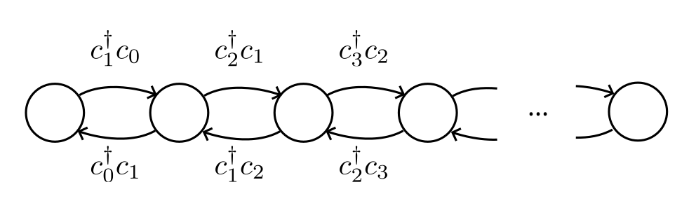
Let us consider the tight-binding Hamiltonian defined on a chain lattice, i.e., the Hamiltonian is given by where is the number of lattice sites, the strength of the hopping term and the annihilation operator at site .
Imports and Parameters
First, we need to import the functions, classes and modules that are required for the script. If you want to follow along, copy the following imports into your script file. We will explain the classes and functions as we go along.
# Title    : HQS Quantum Solver Getting Started Guide
# Filename : fermionic_basics.py

# Python, NumPy, SciPy, and Matplotlib imports
from math import pi, sqrt
import numpy as np
from scipy.linalg import toeplitz, norm
from scipy.sparse.linalg import eigsh
import matplotlib.pyplot as plt

# HQS Quantum Solver imports
from hqs_quantum_solver.spinless_fermions import (
    VectorSpace, Operator, hopping, number, annihilation
)
from hqs_quantum_solver.util import unit_vector
Next, we define the parameters that we will refer to in the script.
M = 16  # site count
N = 1   # particle count
IE = 0  # number of energy level to plot
With that out of the way, we can start setting up the tight-binding Hamiltonian.
Setting up the Hamiltonian
We want to look at a system given by the tight-binding Hamiltonian. Thus, the first step is to construct said Hamiltonian. Quantum Solver provides a generic interface for constructing quantum mechanical operators, as well as several convenience functions.
The first step in constructing an operator is to define the vector space
the operator will be acting on. In quantum mechanics we consider vector
spaces where each basis vector corresponds to a state of the system. Hence, to
define a Quantum Solver vector space, we need to specify the states of the
system. For this particular example, we want the states that have
exactly N particles distributed across M sites. The corresponding
vector space is constructed by creating an instance of the
VectorSpace
in the following way.
v = VectorSpace(sites=M, particle_numbers=N)
Note that Quantum Solver is also able to create vector spaces for a varying number of particles (see spinless_fermions.VectorSpace, HQS Quantum Solver Reference). Fixing the number of particles, however, reduces the amount of memory and computation time Quantum Solver needs.
The second step, is to define the mathematical terms that define the operator.
In Quantum Solver, operators are built by combining multiple mathematical
terms. For the current example, we use the function called
hopping,
which is part of the
spinless_fermions
module, and which implements the term
where is the, so called, hopping matrix.
If we define the matrix to be
then the term in the previous formula becomes the tight-binding
Hamiltonian defined at the beginning of this chapter.
This matrix can be easily constructed using the
toeplitz
function from SciPy in combination with the
unit_vector utility function.
t = 1
h0 = toeplitz(-t * unit_vector(v.sites, 1))
With this matrix at hand, we can construct the Hamiltonian, by passing the term and the vector space defining the operator to the constructor of the Operator class.
H = Operator(hopping(h0), domain=v)
The Quantum Solver operators primarily provide matrix-vector and
matrix-matrix routines and are also directly compatible with most sparse
matrix routines from SciPy. More precisely, most operators, like the one we
have constructed here, implement the methods defined in the
OperatorProtocol
class, as well as the SciPy LinearOperator
interface. As a first example for using the
operator, we want to look at its spectrum. For that, we can directly use
the eigsh
function from SciPy.
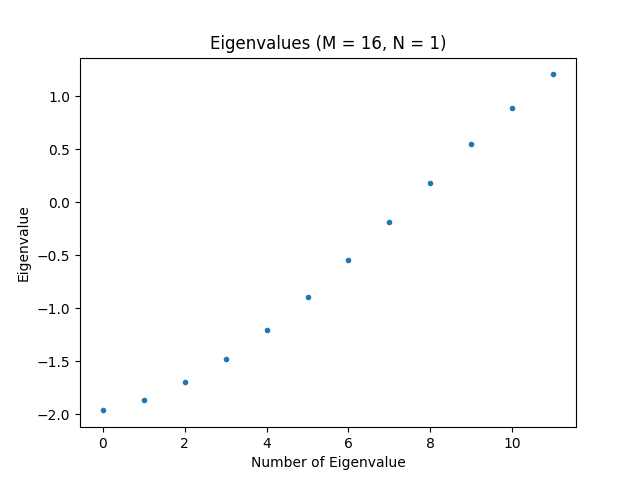
k = min(12, H.shape[0] - 1)  # Number of eigenvalues to compute
evals, evecs = eigsh(H, k=k, which="SA")

print(evals)

plt.figure("eigenvalues", clear=True)
plt.title(f"Eigenvalues (M = {M}, N = {N})")
plt.plot(evals, ".")
plt.xlabel("Number of Eigenvalue")
plt.ylabel("Eigenvalue")
plt.show()
Now, we have enough code to run the script for the first time. Doing so should produce the plot shown below, which shows the ten smallest eigenvalues of the Hamiltonian, and hence, the lowest energy levels of the system.
Before continuing, modify the values of and , run the script, and look at the result a few times.
Note, for a fixed number of particles N the number of states
Quantum Solver has to store is
. Hence, the number of states can grow rather quickly when
increasing N while M is large. This problem gets worse when allowing
the particle number to vary. Keep in mind, while
Quantum Solver provides you with highly accurate computations, you will
have to provide enough computational resources for it to shine.
Below, we have listed the 5 smallest eigenvalues for M = 16 and different
values of N.
| # | |||
|---|---|---|---|
| 1 | -1.97 | -3.83 | -5.53 |
| 2 | -1.86 | -3.67 | -5.31 |
| 3 | -1.70 | -3.57 | -5.14 |
| 4 | -1.48 | -3.44 | -5.04 |
| 5 | -1.21 | -3.34 | -5.04 |
We can make our first observation: Adding the first two values of the column gives you the first value in the column, and adding the first three values of the column will give you the first value in the column. The reason for this is that in a two- and three-particle system of non-interacting paricles, the lowest energy to obtain is the one of the particles occupying the lowest two and three energy levels, respectively. Since we are dealing with a fermionic system, the particles are not allowed to occupy the same state, which explains this behavior.
We shall later come back to this observation.
Note how only few lines of code were necessary to produce physically meaningful results.
Site Occupations
To take this example a little bit further, let us look at the computation of site occupation expectation values. More precisely, we want to compute for , where and
To evaluate this term, we first have to create the number operator for
each site. The
number function, is
provided for this purpose. This function takes the named argument site
and returns the corresponding term.
The term can then be passed to the constructor of the
Operator class,
as we have done for the construction of the Hamiltonian in the previous
section.
Once we have constructed the operator, we can use the
dot
method, to get .
Then we use the
numpy.vdot
function, to compute the scalar product. With this information, we can
write the code that measures the occupation expectation value.
Below, we define a function site_occupation which computes the expectation
value for a given state vector and site. We then plot the expectation
value for every site and for the state vector corresponding to the
energy level IE.
def site_occupation(psi, j):
    number_operator = Operator(number(site=j), domain=v)
    return np.vdot(psi, number_operator.dot(psi))

occupations = np.array([site_occupation(evecs[:, IE], j) for j in range(M)])
plt.figure("site_occupation", clear=True)
plt.title(f"Site Occupation (M = {M}, N = {N}, IE = {IE})")
plt.plot(occupations, "x-")
plt.axis((0, M - 1, 0, 1))
plt.xlabel("j")
plt.ylabel("Expectation Value")
plt.show()
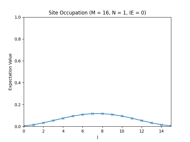
The site occupations for M=16, N=1, IE=0.
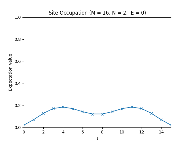
The site occupations for M=16, N=2, IE=0.
Energy occupations
While looking at site occupations is certainly interesting, for most applications it is more useful to look at energy occupations instead.
Consider the matrix given by The columns of this matrix are the eigenvectors of the matrix . It is a well-known fact that if we define we can write the Hamiltonian as where are the energy levels of the system. Consequently, we can measure the expectation value of the occupation of the -th energy level, by computing Note that Hence, we just need to compute and then compute the square norm of this vector.
First, we have to construct the annihilation operator , which is a linear combination of the annihilation operators . The annihilation operator reduces the number of particles in the system by one. In case an operator changes the particle number, in addition to specifying the domain, the codomain needs to be given as well. To construct the codomain vector space, we can use the copy method on the existing vector space to obtain a modified copy.
v_minus = v.copy(particle_number_change=-1)
The term that describes the annihilation operator is given by the
annihilation function.
This function takes the keyword argument site to specify the site at which
to apply the annihilation operator, but, conveniently, also
takes the coef argument, which allows specifying a linear combination
of annihilation operators. Setting coef to the desired linear combination
and then passing this term, the domain, and the codomain to the
constructor of the Operator class constructs the desired operator
. Once the operator is constructed, the computation of the
energy occupation is straightforward.
J, K = np.meshgrid(np.arange(M), np.arange(M), indexing='ij')
Q = sqrt(2) / sqrt(M+1) * np.sin((J+1) * (K+1) * pi / (M+1))

def energy_occupation(psi, k):
    annihilation_operator = Operator(
        annihilation(coef=Q[:,k].conj()), domain=v, codomain=v_minus
    )
    return norm(annihilation_operator.dot(psi))**2

ks = np.arange(M)
expectation = np.array([energy_occupation(evecs[:, IE], k) for k in ks])
plt.figure("energy", clear=True)
plt.title(f"Energy Occupation (M = {M}, N = {N}, IE = {IE})")
plt.plot(ks, expectation, "x-")
plt.xlabel("p")
plt.ylabel("Expectation Value")
plt.show()
Below, you can find the plots that this script produces for different parameter configurations.
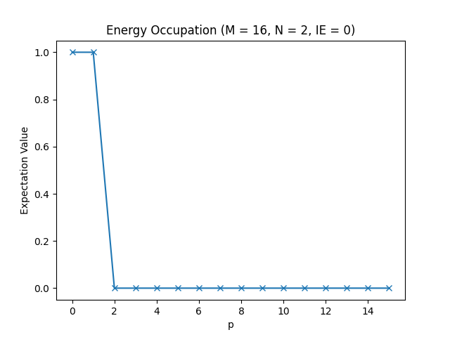
The energy occupations for M=16, N=2, IE=0.
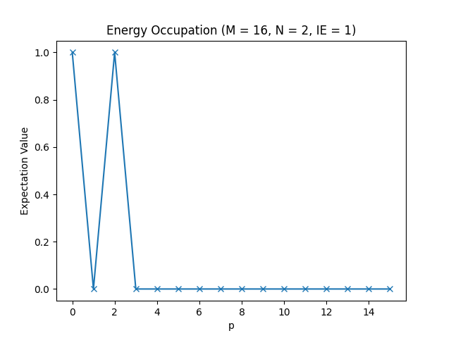
The energy occupations for M=16, N=2, IE=1.
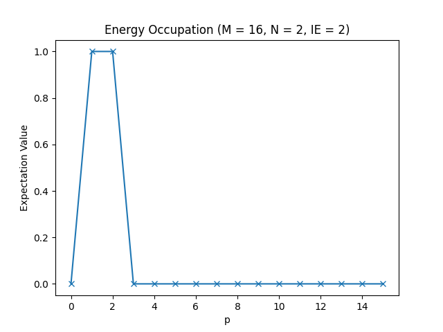
The energy occupations for M=16, N=2, IE=2.
In these figures, you can see how the fermions arrange in the different one-particle energy states to achieve the energy levels we have observed in the table in the Setting up the Hamiltonian section.
Note that if you do not know the eigenvectors of the matrix , you can
easily obtain them by using the
eigh
function of NumPy.
Summary
To conclude this introduction, let us sum up the main takeaways of this chapter.
- Quantum Solver provides classes to work with quantum mechanical operators.
- Operators are constructed by specifying a term and a vector space.
- For operators that change the particle number, the codomain must be given as well.
- Operators provide operations on vectors and matrices (as described in
the OperatorProtocol class),
like the
dotmethod, which applies the operator to a state vector.
Complete Code
# Title    : HQS Quantum Solver Getting Started Guide
# Filename : fermionic_basics.py

# Python, NumPy, SciPy, and Matplotlib imports
from math import pi, sqrt
import numpy as np
from scipy.linalg import toeplitz, norm
from scipy.sparse.linalg import eigsh
import matplotlib.pyplot as plt

# HQS Quantum Solver imports
from hqs_quantum_solver.spinless_fermions import (
    VectorSpace, Operator, hopping, number, annihilation
)
from hqs_quantum_solver.util import unit_vector

# ===== Parameters =====

M = 16  # site count
N = 1   # particle count
IE = 0  # number of energy level to plot

# ===== Creation of the Hamiltonian =====

v = VectorSpace(sites=M, particle_numbers=N)

t = 1
h0 = toeplitz(-t * unit_vector(v.sites, 1))

H = Operator(hopping(h0), domain=v)

# ===== Computing the Eigenvalues and Eigenvectors =====

k = min(12, H.shape[0] - 1)  # Number of eigenvalues to compute
evals, evecs = eigsh(H, k=k, which="SA")

print(evals)

plt.figure("eigenvalues", clear=True)
plt.title(f"Eigenvalues (M = {M}, N = {N})")
plt.plot(evals, ".")
plt.xlabel("Number of Eigenvalue")
plt.ylabel("Eigenvalue")
plt.show()

# ===== Plotting the Site Occupations =====

def site_occupation(psi, j):
    number_operator = Operator(number(site=j), domain=v)
    return np.vdot(psi, number_operator.dot(psi))

occupations = np.array([site_occupation(evecs[:, IE], j) for j in range(M)])
plt.figure("site_occupation", clear=True)
plt.title(f"Site Occupation (M = {M}, N = {N}, IE = {IE})")
plt.plot(occupations, "x-")
plt.axis((0, M - 1, 0, 1))
plt.xlabel("j")
plt.ylabel("Expectation Value")
plt.show()

# ===== Plotting the Energy Occupations =====

v_minus = v.copy(particle_number_change=-1)

J, K = np.meshgrid(np.arange(M), np.arange(M), indexing='ij')
Q = sqrt(2) / sqrt(M+1) * np.sin((J+1) * (K+1) * pi / (M+1))

def energy_occupation(psi, k):
    annihilation_operator = Operator(
        annihilation(coef=Q[:,k].conj()), domain=v, codomain=v_minus
    )
    return norm(annihilation_operator.dot(psi))**2

ks = np.arange(M)
expectation = np.array([energy_occupation(evecs[:, IE], k) for k in ks])
plt.figure("energy", clear=True)
plt.title(f"Energy Occupation (M = {M}, N = {N}, IE = {IE})")
plt.plot(ks, expectation, "x-")
plt.xlabel("p")
plt.ylabel("Expectation Value")
plt.show()
Building Operators
Quantum Solver allows quantum mechanical operators to be constructed in a flexible and convenient way. As we have seen in the "Fermionic Basics" section, quantum mechanical operators are constructed by providing a mathematical term and a vector space. The constructor of the Operator class, however, does not only accept single terms, but arbitrary linear combinations of terms, which makes this interface flexible.
To demonstrate this feature, let us consider the following example. Assume we want to construct the Hamiltonian , where . We start by performing the necessary imports and defining the Parameters.
# NumPy, SciPy, and Matplotlib imports
import numpy as np
from scipy.linalg import toeplitz
from scipy.sparse.linalg import eigsh
import matplotlib.pyplot as plt

# HQS Quantum Solver imports
from hqs_quantum_solver.spinless_fermions import (
    VectorSpace,
    Operator,
    hopping,
    interaction,
    number,
)
from hqs_quantum_solver.util import unit_vector

# ===== Parameters =====

M = 16  # site count
N = 2  # particle count
t = 1  # hopping strength
U = 10  # interaction strength
Then, we create the VectorSpace object, like in the "Fermionic Basics" section, i.e.:
v = VectorSpace(sites=M, particle_numbers=N)
We can now consider the individual parts of the formula for the Hamiltonian. We use the two functions hopping and interaction, which both expect a matrix as input that describes between which sites a particle can move and which pairs of sites expose particles to interactive forces, respectively. The term can be obtained by passing the matrix to the hopping function, and this matrix can be constructed by:
neighbors = toeplitz(unit_vector(v.sites, 1))
The term can be obtained by passing the matrix to the interaction function, and this matrix can be constructed by:
right_neighbors = toeplitz(np.zeros(v.sites), unit_vector(v.sites, 1))
We can now combine the individual terms, to construct the desired Hamiltonian.
H = Operator(-t * hopping(neighbors) + U * interaction(right_neighbors), domain=v)
Using the same code as discussed in the "Fermionic Basics" section, we can compute the expectation value of the occupation for different values of .
# ===== Computing the Eigenvalues and Eigenvectors =====

k = min(12, H.shape[0] - 1)  # Number of eigenvalues to compute
evals, evecs = eigsh(H, k=k, which="SA")
groundstate = evecs[:, 0]

# ===== Plotting the Site Occupations =====

def site_occupation(psi, j):
    n = Operator(number(site=j), domain=v)
    return np.vdot(psi, n.dot(psi))

occupations = np.array([site_occupation(groundstate, j) for j in range(M)])
plt.figure("site_occupation", clear=True)
plt.title(f"Site Occupation (M = {M}, N = {N}, t={t}, U={U})")
plt.plot(occupations, "x-")
plt.axis((0, M - 1, 0, 1))
plt.xlabel("j")
plt.ylabel("Expectation Value")
plt.show()
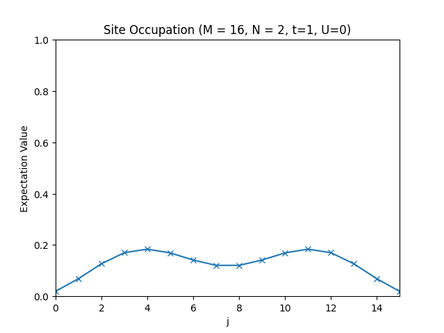
The site occupations for .
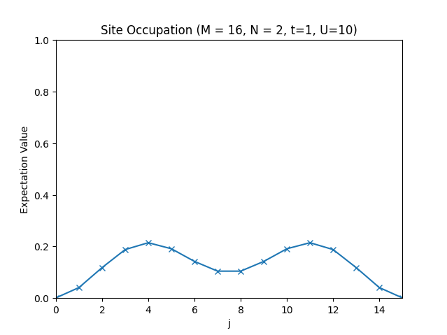
The site occupations for .
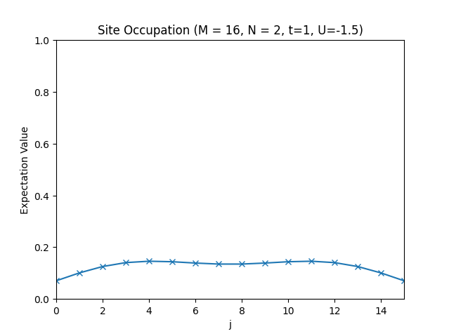
The site occupations for .
Complete Code
# Title    : HQS Quantum Solver Hubbard Interaction
# Filename : hubbard_interaction.py

# NumPy, SciPy, and Matplotlib imports
import numpy as np
from scipy.linalg import toeplitz
from scipy.sparse.linalg import eigsh
import matplotlib.pyplot as plt

# HQS Quantum Solver imports
from hqs_quantum_solver.spinless_fermions import (
    VectorSpace,
    Operator,
    hopping,
    interaction,
    number,
)
from hqs_quantum_solver.util import unit_vector

# ===== Parameters =====

M = 16  # site count
N = 2  # particle count
t = 1  # hopping strength
U = 10  # interaction strength

# ===== Creation of the Hamiltonian =====

v = VectorSpace(sites=M, particle_numbers=N)

neighbors = toeplitz(unit_vector(v.sites, 1))
right_neighbors = toeplitz(np.zeros(v.sites), unit_vector(v.sites, 1))

H = Operator(-t * hopping(neighbors) + U * interaction(right_neighbors), domain=v)

# ===== Computing the Eigenvalues and Eigenvectors =====

k = min(12, H.shape[0] - 1)  # Number of eigenvalues to compute
evals, evecs = eigsh(H, k=k, which="SA")
groundstate = evecs[:, 0]

# ===== Plotting the Site Occupations =====

def site_occupation(psi, j):
    n = Operator(number(site=j), domain=v)
    return np.vdot(psi, n.dot(psi))

occupations = np.array([site_occupation(groundstate, j) for j in range(M)])
plt.figure("site_occupation", clear=True)
plt.title(f"Site Occupation (M = {M}, N = {N}, t={t}, U={U})")
plt.plot(occupations, "x-")
plt.axis((0, M - 1, 0, 1))
plt.xlabel("j")
plt.ylabel("Expectation Value")
plt.show()
System Types
Up until this point, we have only considered quantum mechanical systems
composed of "spinless fermions". HQS Quantum Solver, however, provides
further types of quantum systems. Each of these systems is implemented
in its own module, and all these modules are structured in a similar way,
meaning that they all provide a VectorSpace, an Operator, and a set
of functions providing operator terms.
Spins
The spins module implements systems consisting of spin- particles. The VectorSpace is spanned by vectors of the form As a shorthand, we usually write, e.g.,
With this module, e.g., the
quantum Heisenberg model,
can be simulated. See the spin_waves.ipynb example for details.
Spinless Fermions
The spinless_fermions module implements systems of fermions having a site index but no (dedicated) spin index. The VectorSpace is spanned by vectors of the form and is the creation operator for site .
With this module, e.g., the tight-binding model, can be simulated, as was shown in the "Fermionic Basics" section.
Spinful Fermions
The spinful_fermions module implements system of fermions having a site index and a spin index. The VectorSpace is spanned by vectors of the form and is the creation operator for site and spin polarization .
With this module, e.g., the Hubbard model,
can be simulated. See the spinful_fermions_groundstate.ipynb example for
details.
Bosons
The bosons module implements systems of bosons. The VectorSpace is spanned by vectors of the form and is the creation operator for site . The variable is the maximal occupation of site .
With this module, e.g., the Bose-Hubbard model,
can be simulated. See the bose_hubbard_groundstate.ipynb example for
details.
Advanced Examples
Before looking at the examples, it is advised that you read the Quantum Solver Concepts chapter.
The examples described below can be accessed via HQStage by executing the following shell command.
hqstage download-examples --modules hqs-quantum-solver-examples
The examples available are are listed below.
-
spinful_fermions_groundstate.ipynbIn this example, we show how to compute the ground state of the Hamiltonian of a many-particle system.
-
spin_waves.ipynbThis example introduces spin systems and time evolution. We consider the time evolution of a Heisenberg spin model in an excited state.
-
nonequilibrium_electron_transport.ipynbThis example simulates the time evolution of a system of electrons starting in a nonequilibrium state.
-
spinless_fermions_greens_function.ipynbExample for the Calculation of the Spectral function using HQS Quantum Solver and Lattice Functions.
This method combines operators, Chebyshev expansion, cluster perturbation theory and clever Green's function mathematics to create the reciprocal-space resolved spectral function (a. k. a. the interacting band structure) in a honeycomb lattice causing an opening of the Dirac point.
-
spinful_fermions_greens_function.ipynbPrototype example for the Calculation of the Spectral function of the Hubbard model using HQS Quantum Solver. In this approach we represent the wavefunction as a dyadic product of up and down states.
Similar to the previous example, this example computes the interacting band structure of a square lattice under the influence of interaction. We retrieve the expected behaviour of opening a gap at half-filling.
-
bose_hubbard_groundstate.ipynbIn this example we compute the groundstates of Bose-Hubbard systems, which is a simple bosonic system.
-
lidar.ipynbIn this scientific example we study properties of light emitted by multiple atoms, a fundamental model in quantum optics. We use the HQS Quantum Solver to time evolve the system according to the Lindblad equation of motion and calculate various expectation values of system operators describing properties of the emitted light.
-
advanced_vector_spaces_with_struqture.ipynbIn this example we show how to use the advanced features of the vector space implementations, like combining spaces and tensor products. Furthermore, we use Struqture to describe the operators.
Custom Operators
Many algorithms in HQS Quantum Solver can be used with your own operator implementations. All that is required is that your implementation fulfills the requirements of the protocols used by the algorithm of interest.
Protocols
Protocols are a Python language feature that allows describing the requirements an object has to fulfill for being used in a particular part of the program. Whenever you encounter a protocol class in the type hints of a function or method, the protocol class defines which methods and properties the corresponding argument object is expected to have and the corresponding return type it has to provide, respectively. It is not necessary that your class inherits from the protocol class.
For example, the
evolve_krylov function
expects a operator argument which adheres to the
SimpleOperatorProtocol.
To be allowed to pass an object as operator, the object just needs
to implement all the methods and properties listed in
SimpleOperatorProtocol,
which are the shape and dtype attributes and the dot method.
Example
In this example we want to simulate the time evolution of a single spin in a magnetic field for different field stengths, i.e, we consider the Hamiltonian for different values of and measure the expectation value of . Instead of building a new operator for every value of we are interested in, we create a Hamiltonian class, that applies the correct value of on the fly. Avoiding recreation of operators can sometimes reduce the time of the computation. For a single-spin system, however, we will not see any benefit, because the system is too small. Nevertheless, we stick with this simple example for demonstration purposes.
We start by performing the necessary imports.
# Title    : HQS Quantum Solver Larmor Precession
# Filename : larmor_precession.py
import numpy as np
from scipy.sparse.linalg import eigsh
import matplotlib.pyplot as plt
from hqs_quantum_solver.spins import VectorSpace, Operator, spin_x, spin_z
from hqs_quantum_solver.evolution import evolve_krylov, observers
Next, we construct the and operators, and we set the initial state to an eigenvalue of the operator.
v = VectorSpace(sites=1, total_spin_z="all")
Sx = Operator(spin_x(site=0), domain=v)
Sz = Operator(spin_z(site=0), domain=v)

eigvals, eigvecs = eigsh(Sx, k=1)
state = eigvecs[:, 0]
We can now define the Hamiltonian class as a custom operator.
In this class, we need to define the shape and dtype property and
the dot method. Note that the implementation of the dot method
is required to have a parameter called out that when not equal to
None needs to be filled with the result of the operator application.
class Hamiltonian:
    def __init__(self, B):
        self.B = B

    @property
    def shape(self):
        return Sz.shape

    @property
    def dtype(self):
        return Sz.dtype

    def dot(self, x, out=None):
        result = -self.B * Sz.dot(x)
        if out is not None:
            np.copyto(out, result)
        return result
We can now pass instances of the Hamiltonian class to the evolve_krylov function, like any other operator provided by HQS Quantum Solver.
times = np.linspace(0, 1, 100)

Bs = [1, 2, 5, 10]
observations = np.empty((len(Bs), times.size))
for n in range(len(Bs)):
    B = Bs[n]
    result = evolve_krylov(Hamiltonian(B=B), state, times, observer=observers.expectation([Sx]))
    observations[n, :] = np.array(result.observations)[:, 0]

plt.plot(
    times, observations[0, :],
    times, observations[1, :],
    times, observations[2, :],
    times, observations[3, :],
)
plt.legend([f"$B = {B}$" for B in Bs])
plt.xlabel(r"$t$")
plt.ylabel(r"$\langle S^x \rangle$")
plt.show()
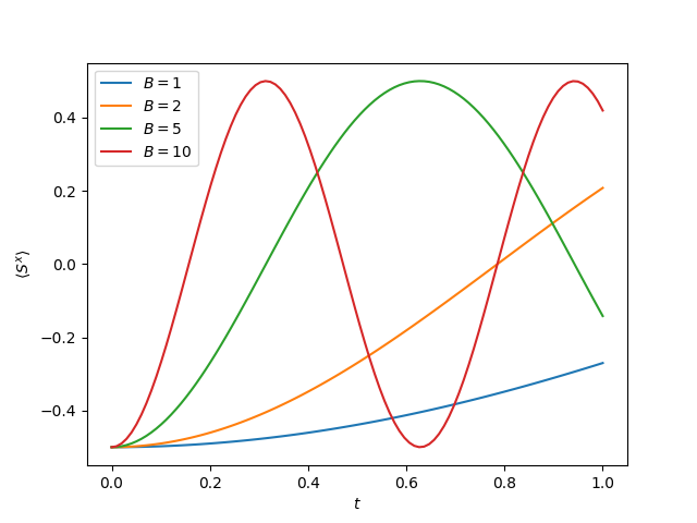
The expectation value of measuring .
Complete Code
# Title    : HQS Quantum Solver Larmor Precession
# Filename : larmor_precession.py
import numpy as np
from scipy.sparse.linalg import eigsh
import matplotlib.pyplot as plt
from hqs_quantum_solver.spins import VectorSpace, Operator, spin_x, spin_z
from hqs_quantum_solver.evolution import evolve_krylov, observers

v = VectorSpace(sites=1, total_spin_z="all")
Sx = Operator(spin_x(site=0), domain=v)
Sz = Operator(spin_z(site=0), domain=v)

eigvals, eigvecs = eigsh(Sx, k=1)
state = eigvecs[:, 0]

class Hamiltonian:
    def __init__(self, B):
        self.B = B

    @property
    def shape(self):
        return Sz.shape

    @property
    def dtype(self):
        return Sz.dtype

    def dot(self, x, out=None):
        result = -self.B * Sz.dot(x)
        if out is not None:
            np.copyto(out, result)
        return result

times = np.linspace(0, 1, 100)

Bs = [1, 2, 5, 10]
observations = np.empty((len(Bs), times.size))
for n in range(len(Bs)):
    B = Bs[n]
    result = evolve_krylov(Hamiltonian(B=B), state, times, observer=observers.expectation([Sx]))
    observations[n, :] = np.array(result.observations)[:, 0]

plt.plot(
    times, observations[0, :],
    times, observations[1, :],
    times, observations[2, :],
    times, observations[3, :],
)
plt.legend([f"$B = {B}$" for B in Bs])
plt.xlabel(r"$t$")
plt.ylabel(r"$\langle S^x \rangle$")
plt.show()
Lattice Builder
When building Hamiltonians with Quantum Solver, it is often required to create adjacency matrices that represent the lattice structure of the system under consideration, e.g., for the hopping term. Building those terms in 1d is relatively straight forward. For higher dimensions and more complicated lattices, however, this becomes more difficult. The HQS Lattice Builder and Lattice Validator are libraries that simplify this process and can directly be used with Quantum Solver.
As an example, we consider the computation of the groundstate of the tight-binding Hamiltonian, but this time on a rectangular lattice. The Hamiltonian is given by where is the set of all tuples such that is a neighbor of .
We start the example by specifying the required imports.
# NumPy, SciPy, and Matplotlib imports
import numpy as np
from scipy.sparse.linalg import eigsh
import matplotlib.pyplot as plt

# HQS Quantum Solver imports
from hqs_quantum_solver.spinless_fermions import (
    VectorSpace, Operator, lattice_term, annihilation
)

# HQS Lattice Builder/Validator imports
import lattice_builder
import lattice_validator
Then, we define the parameters of the simulation.
Mx = 5  # sites in x-direction
My = 4  # sitex in y-direction
N = 1  # particle count
t = 1  # hopping strengh
The next step is to create a Lattice Builder/Validator configuration
that specifies the Hamiltonian on an Mx My rectangular lattice.
In this example we have just one type of atom (lattice site) that is
repeated in the direction of the vectors in "lattice_vectors".
The hopping term is defined in the bonds variable, which adds an entry
of value -t into the hopping matrix for neighboring lattice sites.
For more details on the Lattice Builder configuration, take a look at the Hamiltonians in "Physics", HQS Lattice Documentation documentation, and at "Schema definitions", Lattice Validator Documentation.
system = {
    "site_type": "spinless_fermions",
    "cluster_size": [Mx, My, 1],
    "system_boundary_conditions": ["hard-wall", "hard-wall", "hard-wall"]
}
atoms = [{"id": 0}]
bonds = [
    {"id_from": 0, "id_to": 0, "translation": [1, 0, 0], "t": -t},
    {"id_from": 0, "id_to": 0, "translation": [0, 1, 0], "t": -t},
]
unitcell = {
    "atoms": atoms,
    "bonds": bonds,
    "lattice_vectors": [[1, 0, 0], [0, 1, 0]]
}
conf = {
    "system": system,
    "unitcell": unitcell
}
The configuration needs to be validated and normalized, which is done by using the Lattice Validator. Then, a Lattice Builder instance can be created. This instance is then passed to the lattice_term function, to convert it into an operator definition.
Note, if you do not need access to the Lattice Builder instance, you can also
directly pass the conf dict to lattice_term, which will take care of
the validation and builder construction.
is_valid, conf = lattice_validator.Validator().validateConfiguration(conf)
if not is_valid:
    raise ValueError(f"Configuration not valid: {conf}")
builder = lattice_builder.Builder(conf)

v = VectorSpace(sites=Mx * My, particle_numbers=N)
H = Operator(lattice_term(builder), domain=v)
After having obtained the Hamiltonian operator, the computation of the
groundstate and the definition of the site_occupation function are
the same as in the "Fermionic Basics" section.
k = min(12, H.shape[0] - 1)  # Number of eigenvalues to compute
evals, evecs = eigsh(H, k=k, which="SA")
groundstate = evecs[:, 0]

v_minus = v.copy(particle_number_change=-1)

def site_occupation(psi, j):
    annihilation_operator = Operator(annihilation(site=j), domain=v, codomain=v_minus)
    c_psi = annihilation_operator.dot(psi)
    return c_psi.conj() @ c_psi
To plot the result we use the get_atom_positions method from the Lattice
Builder to show the groundstate occupation on a 2d grid.
occupations = np.zeros((My, Mx))
for j, position in enumerate(builder.get_atom_positions().tolist()):
    x, y = round(position[0]), round(position[1])
    # Set value for row=y and column=x.
    occupations[y, x] = site_occupation(groundstate, j)

plt.figure("site_occupation", clear=True)
plt.title(f"Site Occupation (lattice: {Mx}x{My}, particles: {N})")
plt.imshow(occupations, origin="lower", aspect="equal")
plt.xlabel("x")
plt.ylabel("y")
plt.xticks(np.arange(Mx))
plt.yticks(np.arange(My))
plt.colorbar()
plt.show()
Finally, we can run the code, to obtain a plot of the occupation, as shown below.
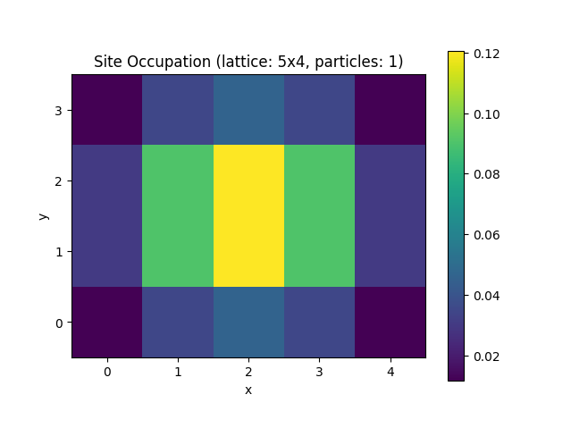
Complete Code
# Title    : HQS Quantum Solver using the Lattice Builder
# Filename : getting_started.py

# NumPy, SciPy, and Matplotlib imports
import numpy as np
from scipy.sparse.linalg import eigsh
import matplotlib.pyplot as plt

# HQS Quantum Solver imports
from hqs_quantum_solver.spinless_fermions import (
    VectorSpace, Operator, lattice_term, annihilation
)

# HQS Lattice Builder/Validator imports
import lattice_builder
import lattice_validator

# ===== Parameters =====

Mx = 5  # sites in x-direction
My = 4  # sitex in y-direction
N = 1  # particle count
t = 1  # hopping strengh

# ===== Definition of the Lattice =====

system = {
    "site_type": "spinless_fermions",
    "cluster_size": [Mx, My, 1],
    "system_boundary_conditions": ["hard-wall", "hard-wall", "hard-wall"]
}
atoms = [{"id": 0}]
bonds = [
    {"id_from": 0, "id_to": 0, "translation": [1, 0, 0], "t": -t},
    {"id_from": 0, "id_to": 0, "translation": [0, 1, 0], "t": -t},
]
unitcell = {
    "atoms": atoms,
    "bonds": bonds,
    "lattice_vectors": [[1, 0, 0], [0, 1, 0]]
}
conf = {
    "system": system,
    "unitcell": unitcell
}

# ===== Creation of the Hamiltonian =====

is_valid, conf = lattice_validator.Validator().validateConfiguration(conf)
if not is_valid:
    raise ValueError(f"Configuration not valid: {conf}")
builder = lattice_builder.Builder(conf)

v = VectorSpace(sites=Mx * My, particle_numbers=N)
H = Operator(lattice_term(builder), domain=v)

# ===== Computing the Eigenvalues and Eigenvectors =====

k = min(12, H.shape[0] - 1)  # Number of eigenvalues to compute
evals, evecs = eigsh(H, k=k, which="SA")
groundstate = evecs[:, 0]

# ===== Plotting the Site Occupations =====

v_minus = v.copy(particle_number_change=-1)

def site_occupation(psi, j):
    annihilation_operator = Operator(annihilation(site=j), domain=v, codomain=v_minus)
    c_psi = annihilation_operator.dot(psi)
    return c_psi.conj() @ c_psi

occupations = np.zeros((My, Mx))
for j, position in enumerate(builder.get_atom_positions().tolist()):
    x, y = round(position[0]), round(position[1])
    # Set value for row=y and column=x.
    occupations[y, x] = site_occupation(groundstate, j)

plt.figure("site_occupation", clear=True)
plt.title(f"Site Occupation (lattice: {Mx}x{My}, particles: {N})")
plt.imshow(occupations, origin="lower", aspect="equal")
plt.xlabel("x")
plt.ylabel("y")
plt.xticks(np.arange(Mx))
plt.yticks(np.arange(My))
plt.colorbar()
plt.show()
API Reference
You are being redirected. If the redirect does not work, click here.