Building Operators
Quantum Solver allows quantum mechanical operators to be constructed in a flexible and convenient way. As we have seen in the "Fermionic Basics" section, quantum mechanical operators are constructed by providing a mathematical term and a vector space. The constructor of the Operator class, however, does not only accept single terms, but arbitrary linear combinations of terms, which makes this interface flexible.
To demonstrate this feature, let us consider the following example. Assume we want to construct the Hamiltonian , where . We start by performing the necessary imports and defining the Parameters.
# NumPy, SciPy, and Matplotlib imports
import numpy as np
from scipy.linalg import toeplitz
from scipy.sparse.linalg import eigsh
import matplotlib.pyplot as plt

# HQS Quantum Solver imports
from hqs_quantum_solver.spinless_fermions import (
    VectorSpace,
    Operator,
    hopping,
    interaction,
    number,
)
from hqs_quantum_solver.util import unit_vector

# ===== Parameters =====

M = 16  # site count
N = 2  # particle count
t = 1  # hopping strength
U = 10  # interaction strength
Then, we create the VectorSpace object, like in the "Fermionic Basics" section, i.e.:
v = VectorSpace(sites=M, particle_numbers=N)
We can now consider the individual parts of the formula for the Hamiltonian. We use the two functions hopping and interaction, which both expect a matrix as input that describes between which sites a particle can move and which pairs of sites expose particles to interactive forces, respectively. The term can be obtained by passing the matrix to the hopping function, and this matrix can be constructed by:
neighbors = toeplitz(unit_vector(v.sites, 1))
The term can be obtained by passing the matrix to the interaction function, and this matrix can be constructed by:
right_neighbors = toeplitz(np.zeros(v.sites), unit_vector(v.sites, 1))
We can now combine the individual terms, to construct the desired Hamiltonian.
H = Operator(-t * hopping(neighbors) + U * interaction(right_neighbors), domain=v)
Using the same code as discussed in the "Fermionic Basics" section, we can compute the expectation value of the occupation for different values of .
# ===== Computing the Eigenvalues and Eigenvectors =====

k = min(12, H.shape[0] - 1)  # Number of eigenvalues to compute
evals, evecs = eigsh(H, k=k, which="SA")
groundstate = evecs[:, 0]

# ===== Plotting the Site Occupations =====

def site_occupation(psi, j):
    n = Operator(number(site=j), domain=v)
    return np.vdot(psi, n.dot(psi))

occupations = np.array([site_occupation(groundstate, j) for j in range(M)])
plt.figure("site_occupation", clear=True)
plt.title(f"Site Occupation (M = {M}, N = {N}, t={t}, U={U})")
plt.plot(occupations, "x-")
plt.axis((0, M - 1, 0, 1))
plt.xlabel("j")
plt.ylabel("Expectation Value")
plt.show()
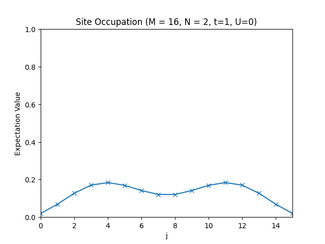
The site occupations for .
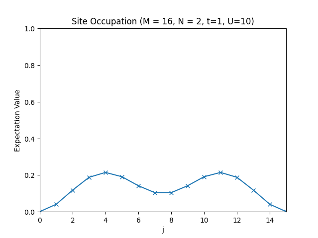
The site occupations for .
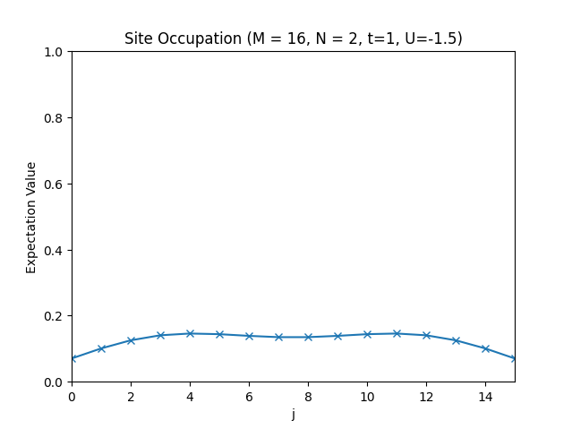
The site occupations for .
Complete Code
# Title    : HQS Quantum Solver Hubbard Interaction
# Filename : hubbard_interaction.py

# NumPy, SciPy, and Matplotlib imports
import numpy as np
from scipy.linalg import toeplitz
from scipy.sparse.linalg import eigsh
import matplotlib.pyplot as plt

# HQS Quantum Solver imports
from hqs_quantum_solver.spinless_fermions import (
    VectorSpace,
    Operator,
    hopping,
    interaction,
    number,
)
from hqs_quantum_solver.util import unit_vector

# ===== Parameters =====

M = 16  # site count
N = 2  # particle count
t = 1  # hopping strength
U = 10  # interaction strength

# ===== Creation of the Hamiltonian =====

v = VectorSpace(sites=M, particle_numbers=N)

neighbors = toeplitz(unit_vector(v.sites, 1))
right_neighbors = toeplitz(np.zeros(v.sites), unit_vector(v.sites, 1))

H = Operator(-t * hopping(neighbors) + U * interaction(right_neighbors), domain=v)

# ===== Computing the Eigenvalues and Eigenvectors =====

k = min(12, H.shape[0] - 1)  # Number of eigenvalues to compute
evals, evecs = eigsh(H, k=k, which="SA")
groundstate = evecs[:, 0]

# ===== Plotting the Site Occupations =====

def site_occupation(psi, j):
    n = Operator(number(site=j), domain=v)
    return np.vdot(psi, n.dot(psi))

occupations = np.array([site_occupation(groundstate, j) for j in range(M)])
plt.figure("site_occupation", clear=True)
plt.title(f"Site Occupation (M = {M}, N = {N}, t={t}, U={U})")
plt.plot(occupations, "x-")
plt.axis((0, M - 1, 0, 1))
plt.xlabel("j")
plt.ylabel("Expectation Value")
plt.show()