Introduction
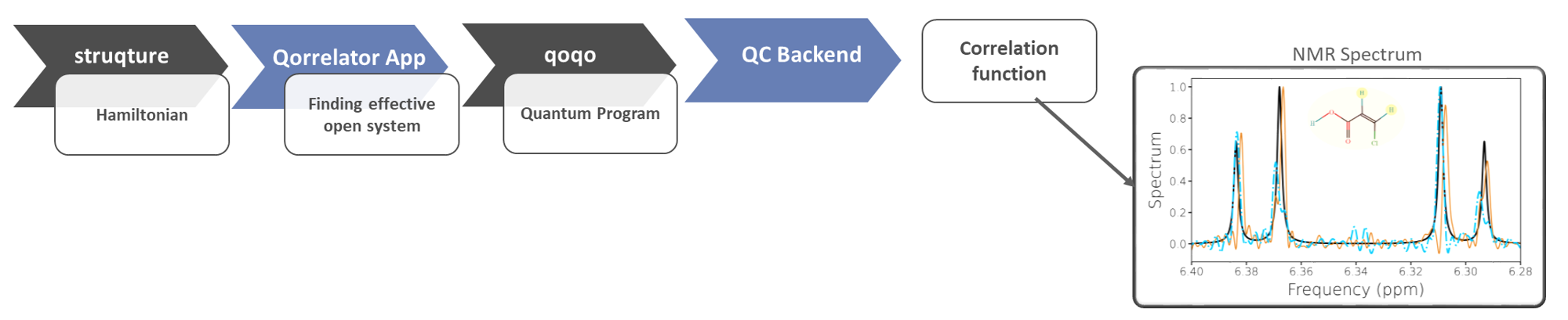
HQS Qorrelator App is a user-friendly solution designed to calculate correlation functions using quantum computers.
Correlation functions, and the response spectra that can be calculated from them, are the vital connection between the macroscopic and the microscopic world in physics and chemistry. For example, in chemistry spectroscopy and most importantly Nuclear Magnetic Resonance (NMR)-spectroscopy is an irreplaceable tool to identify chemical compounds. In physics correlation functions of materials (for example the Green’s function) determine how a material responds to external drives like electric fields or currents and are the standard object of interest for almost all work on quantum models like the Hubbard model.
The calculation of correlation functions is one of the earliest use cases where a quantum advantage can be expected. It is based on implementing a quantum time evolution on a quantum computer and sampling from the result. It is vital for users that need to work with correlation functions and response spectra to understand when quantum computers have matured enough to provide a quantum advantage for their use case and how that quantum advantage can be utilized.
The HQS Qorrelator App is designed to provide users with a simple tool to perform the calculation of correlation functions on a quantum computer without being experts in quantum computing. It can be used to benchmark correlation function calculations on current quantum hardware and the potential performance of error corrected quantum computers by using simulators.
Applications
The first version of the HQS Qorrelator App focuses on calculating the NMR correlation functions on a quantum computer. We focus on NMR for two reasons:
- It is hard to overstate the relevance of NMR in experimentally identifying the molecules present in chemical samples and the number of applications of NMR in industry. It is a commercially highly relevant application.
- In the case of standard NMR it is effectively possible to calculate the correlation function in the infinite temperature limit. In this limit the calculation of a correlation function on a quantum computer simplifies further and is essentially reduced to applying the correct time evolution. This makes NMR an excellent candidate for achieving a quantum advantage.
The NMR spectral function can be obtained from the correlation functions of two spin operators, with respect to the Hamiltonian of the nuclear spins targeted by the NMR measurement. The Qorrelator App will take a description of the Hamiltonian and of the quantum device the calculation should run on as an input. It will return a QuantumProgram a collection of quantum circuits and measurement postprocessing needed to calculate the correlation function with a quantum computer. This QuantumProgram can be run on one of several backends and return the correlation function. The spectral function can be obtained from the correlation function with a simple Fourier transform.
In the near future, all available quantum computers will be NISQ quantum computers, where the qubits of the quantum computer experience environmental noise. In most applications, environmental noise is purely a source of errors. At HQS, we have realized that, for certain applications, environmental noise is not detrimental and can even be used as a computational resource.
The HQS Qorrelator App also incorporates these approaches in a user-friendly manner, by providing an easy way to obtain an estimate of the spectral broadening due to the effective time evolution that occurs on a noisy quantum computer.
Getting started
The following command can be used to install the package via hqstage the HQS tool for managing our proprietary software:
hqstage install hqs_qorrelator_app
The usage section breaks down how the HQS Qorrelator App works together with the HQS struqture and qoqo libraries. We go through the Python interface of the package and discuss how to construct quantum programs that will calculate correlations, how to get an estimated broadening based on the noise in a device and how to extract the noisy algorithm model.
The following code snippet provides a basic example. For more details see
# Import tools
import numpy as np
from qoqo import devices
from qoqo_quest import Backend
from struqture_py import spins
from hqs_qorrelator_app import NMRCorrelator

# Creating a Quantum device the calculation should run on
device = devices.AllToAllDevice(
    number_qubits,
    ["RotateZ", "RotateX", "RotateY", "PauliX", "Hadamard", "SingleQubitGate"],
    ["CNOT", "Qsim", "SWAP"],
    1.0,
)
device = device.add_depolarising_all(1e-5)

# Constructing the NMR hamiltonian
hamiltonian = spins.PauliHamiltonian()
# Shifting the second spin by energy 1
hamiltonian.set("1Z", 1)
# Adding a small ZZ interaction between spins
hamiltonian.set("0Z1Z", 1e-3)
# Creating the QuantumProgram
nmr = NMRCorrelator()
program = nmr.spectrum_program_fixed_step(
    hamiltonian, trotter_timestep=0.1, gyromagnetic_factors=[1,1], device=device
)
# Evaluate the program for the correlator after 2 Trotter steps
backend = Backend(number_qubits=2)
res = program.run(backend, [2])
print("Correlation after two trotter steps", res["correlator_total_re"])
Features
The HQS Qorrelator App has the following features:
- Construct a QuantumProgram specific for NMR.
- Construct a QuantumProgram for measuring correlators in infinite temperature environment.
- Create a noise algorithm model for time evolution in correlator measurement.
- Extract the infinite temperature fidelity from a noise model (how well noise model fits infinite temperature assumption).
- Full Python interface.
For experts in quantum computing more features are available when manually constructing quantum programs using the HQS Quantum Libraries.
API Documentation
Changelog
For a changelog starting from version 0.2 please see here.
Installation
The software is delivered in the form of pre-compiled python packages (wheel) qorrelator-app-py.
The python packages have been built for Python versions 3.7 to 3.12 and are compatible with glibc based linux distributions that conform to the manylinux2014 standard.
The software can be installed based on the wheel with
pip install --find-links ./wheels --upgrade qorrelator_app_py
The qorrelator-app has minimal dependencies. All dependencies are open source and available on the public PyPI server. Dependencies should be automatically installed by the above pip command.
General dependencies
HQS dependencies
- qoqo_calculator_pyo3: A simple symbolic value library for qoqo and struqture.
- qoqo: The HQS quantum computing toolkit.
- struqture_py: An HQS library to represent quantum mechanical operators, hamiltonians and open systems.
Using the HQS Qorrelator App
In this section, we outline how to employ the HQS Qorrelator App to compute time-resolved
correlators for NMR spectroscopy simulations on quantum computers. The HQS Qorrelator App works
together with the HQS struqture and
qoqo libraries. In this regard, we first briefly
show how to create Hamiltonians and open quantum systems using struqture. Then, we discuss the
available qoqo noise models that can be used in the simulation, and we show how to set up device
information. Finally, we illustrate how to use the HQS Qorrelator App to create a qoqo
QuantumProgram for simulating the dynamics of the correlators.
struqture
struqture is a library enabling compact representation of quantum mechanical operators, Hamiltonians, and open quantum systems. The library supports building spin, fermionic and bosonic objects, as well as combinations thereof (mixed systems). Here, we demonstrate its usage with simple spin systems. For more complicated examples, please check the user documentation of struqture.
Creating Spin Hamiltonians
Let us now create a NMR Hamiltonian using the struqture library. Struqture uses Pauli Hamiltonians, the only
difference to a Spin Hamiltonian from physics are missing factors of (\frac{1}{2}) for the X, Y and Z operators.
Arbitrary Pauli Hamiltonians are built from PauliProduct operators. As the name implies, these are products of single-spin Pauli
operators. Each Pauli operator in the PauliProduct operates on a different spin. Not all spins
need to be represented in a PauliProduct (such spins contribute via identity operators).
For instance, let us create a simple Hamiltonian in the rotating-wave approximation with respect to
a strong external magnetic field in the Z-direction. Such a Hamiltonian is also required as the input
for constructing the QuantumProgram used to calculate the NMR correlation function. All single-spin
terms need to be Z-terms. All spin-interaction terms need to be at least spin-Z preserving (only
XX, YY or ZZ terms, with the same coefficient for XX and YY) or completely symmetric in X,
Y and Z (same coefficient for XX, YY and ZZ). The second kind of symmetry is required when
setting the b_field_direction option to a different direction from the input Hamiltonian.
For instance, we can create the following Hamiltonian
using:
from struqture_py import spins
from struqture_py.spins import PauliHamiltonian, PauliProduct

number_spins = 10
chemical_shift = 3.0
spin_coupling = 2.0

hamiltonian = PauliHamiltonian()
for site in range(number_spins):
    # Accounting for the factor of 1/2
    hamiltonian.set(f"{site}Z", chemical_shift * 0.5)
for site in range(number_spins - 1):
    hamiltonian.set(f"{site}Z{site+1}Z", spin_coupling*0.5**2)
    hamiltonian.set(f"{site}X{site+1}Y", spin_coupling*0.5**2)
    hamiltonian.set(f"{site}X{site+1}Y", spin_coupling*0.5**2)
Information can be accessed using the following functions:
hamiltonian.keys()                  # operator keys (Pauli products / strings)
hamiltonian.get("0X1X")             # prefactor of Pauli product "0X1X"
hamiltonian.current_number_spins()  # number of spins in the system
Creating a device
To construct a QuantumProgram to calculate a correlation function we need to specify what kind
of device should be used for the calculation. Devices can be specified with the help of the open-source
qoqo library. We will use the simple AllToAllDevice device as an example. For more information about
setting up more complicated devices, please have a look at qoqo.
We can define an AllToAllDevice device with the following settings:
number_qubits: The number of qubits for the device.single_qubit_gates: The list of single-qubit gates available on the quantum computer.two_qubit_gates: The list of two-qubit gates available on the quantum computer.default_gate_time: The default starting gate time.
The option single_qubit_gates can be any list of single-qubit gates available in
qoqo as long as it contains one of the following
combinations:
RotateXandRotateZRotateYandRotateZRotateXandRotateYRotateZandSqrtPauliXandInvSqrtPauliX
The supported choices for two_qubit_gates are:
CNOTControlledPauliZControlledPhaseShiftMolmerSorensenXXVariableMSXX
An example code snippet of setting device information reads as follows.
from qoqo import devices

# Setting up the device.
number_qubits = 10
single_qubit_gates = ["RotateX", "RotateZ", "RotateY"]
two_qubit_gates = ["CNOT"]
default_gate_time = 1.0
device = devices.AllToAllDevice(
    number_qubits, single_qubit_gates, two_qubit_gates, default_gate_time
)
Using the HQS Qorrelator App for calculating NMR correlators
QuantumPrograms for NMR correlation functions are best obtained from the NMRCorrelator class. The NMRCorrelator class can be initialized without any arguments:
from hqs_qorrelator_app import NMRCorrelator

correlator = NMRCorrelator()
Additionally, there are settings that have default values and can be set with setter functions with the same name as the setting.
algorithm: options areParityBased,QSWAP,QSWAPMolmerSorensen,VariableMolmerSorensen(defaults toQSWAP).b_field_direction:Z(default) andXare possible options. Determines in which direction of the B-field is used for the calculation of the correlator. Automatically transforms compatible input Hamiltonians (e.g. a input Hamiltonian defined for aZb-field if theXdirection is used).parallelization_blocks: the way noise is added to a quantum circuit. By default, this is set tofalse, so the noise will be inserted on all qubits after each operation, according to the user-specifiedNoiseModels(see the section onCreating a noise model, below). If theparallelization_blocksoption is set totrue, the noise mode is changed toParallelizationBlocks. In this case, the quantum circuits created are automatically parallelized into blocks that can be executed simultaneously and the noise model adds noise on the qubits that are involved in a parallel block after each block. This noise is added after aPragmaStopParallelBlockthat notifies the end of the parallel operations in a qoqo circuit.number_measurements: the number of projective measurements used when measuring observables (defaults to 100000)initialisation: At the moment available initialisations areSumOverAllStates(default),PositiveMagnetization,RandomStates. See also the chapter on algorithms.
The NMRCorrelator can create QuantumPrograms to time-propagate a spin state. The
QuantumProgram will initialize a spin state on a quantum computer, time-propagate the spin state
with a quantum algorithm, measure the values of spin observables and compute the NMR correlator as
described in the Quantum Algorithm section. The following example
shows how to obtain the QuantumProgram for a previously defined hamiltonian (hamiltonian) and
device (device).
from hqs_qorrelator_app import NMRCorrelator

trotter_timestep = 0.005
gyromagnetic_factors = [1.0] * number_qubits

correlator = NMRCorrelator()
program = correlator.spectrum_program_fixed_step(
    hamiltonian,
    trotter_timestep,
    gyromagnetic_factors,
    device
)
The QuantumProgram can then be simulated using the backend of the user’s choosing.
The qoqo-quest Backend is recommended for simulations. The following example shows how to run the
obtained QuantumProgram on the backend and get the real and imaginary parts of the NMR correlator
from the resulting dictionary.
import numpy as np
from qoqo_quest import Backend

number_trottersteps = 100
backend = Backend(number_qubits)

correlator_re = np.zeros(number_trottersteps, dtype=float)
correlator_im = np.zeros(number_trottersteps, dtype=float)

for i in range(0, number_trottersteps):
    # Time is always propagated in units of the trotter timestep
    # chosen as an input for the quantum program creation
    result = backend.run_program(program, [i])
    correlator_re[i] = result["correlator_total_re"]
    correlator_im[i] = result["correlator_total_im"]

correlator = correlator_re + 1.0j * correlator_im
Considering the effects of noise
In the NISQ era, quantum computers all suffer from physical background noise. In the calculation of correlation functions this leads to an overall decay of the correlation with time and in the resulting spectral function to a broadening of the spectral peaks. Depending on the level of noise these effects can still be acceptable. To better understand the effects of noise and to judge if it is too high to have a chance to obtain good results the HQS Qorrelator app provides methods to calculate the influence of noise on the QuantumProgram running on the noisy quantum computer.
Creating noise models
The current version of the HQS Qorrelator App supports single-qubit physical noise in the form of damping, dephasing, and depolarisation, with user-given decoherence rates. We assume that the noise is the same for all gate-types.
Just like the devices, the noise models are defined with the help of the qoqo library, for more detailed information
about available noise models also see the qoqo repository.
We can define a ContinuousDecoherenceModel a noise model for noise that is always on in the background during the quantum operations.
This noise model supports the following types of noise:
- dephasing: using the
add_dephasing_ratefunction - depolarisation: using the
add_depolarising_ratefunction - damping: using the
add_damping_ratefunction - excitations: using the
add_excitation_ratefunction
Each of these functions takes a list of qubits to apply the noise to, as well as a noise rate (float), and
returns the modified ContinuousDecoherenceModel. An example code snippet, which creates a noise model with
damping and dephasing, reads as follows.
from qoqo import noise_models

# Setting up the noise model.
damping = 1e-3
dephasing = 5e-4
noise_model = noise_models.ContinuousDecoherenceModel().add_damping_rate([0, 1, 2], damping).add_dephasing_rate([3, 4], dephasing)
Estimating the overall decoherence rate
Physical noise on the quantum computer used to run the QuantumProgram will lead to a decay in the calculated correlation functions. This decay will lead to a broadening in the NMR spectrum (the Fourier transform of the correlation function).
Based on the choice of algorithm, device specification, and noise models, the mean decoherence rate that affects the spin system during the time evolution can be estimated. This estimated decoherence rate gives an expected broadening of the peaks in the NMR spectrum.
Please note that this is just an estimate, and therefore does not require a computationally costly full simulation of the time evolution.
from hqs_qorrelator_app import NMRCorrelator
from struqture_py import spins
from qoqo import devices, noise_models

# define hamiltonian
gyromagnetic = 1.0
number_spins = 2
time = np.pi / 4
coupling = 1.0
shift = 1.0
gyromagnetic_factors = [gyromagnetic for _ in range(number_qubits)]
hamiltonian = spins.PauliHamiltonian()
for site in range(number_spins):
    hamiltonian.set("{}Z".format(site), -shift * site)

# Setting up the device.
single_qubit_gates = ["RotateX", "RotateZ", "RotateY"]
two_qubit_gates = ["CNOT"]
gate_times = 1.0
damping = 1e-3
device = devices.AllToAllDevice(number_spins, single_qubit_gates, two_qubit_gates, gate_times)
# While the noise model is not needed to generate the QuantumProgram, it will be required
# when simulating the QuantumProgram.
noise_model = noise_models.ContinuousDecoherenceModel().add_damping_rate([0, 1, 2], damping)

trotter_timestep = 0.01

# Create circuit.
qorrelator_app_sc = NMRCorrelator()
qorrelator_app_sc.algorithm = "QSWAP"
estimated_decoherence_rate = qorrelator_app_sc.estimate_decoherence_rate(
    hamiltonian, trotter_timestep, device, [noise_model]
)

print("estimated decoherence rate:", estimated_decoherence_rate)
Extracting the Noisy algorithm model
The noisy algorithm model represents the effective Lindbladian that is being simulated in the presence of noise. Please refer to this paper and to the mapping section for details.
With the HQS Qorrelator App, the noisy algorithm model of a Hamiltonian can be obtained using the
function NMRCorrelator.noisy_algorithm_model, with input arguments:
hamiltonian: The Hamiltonian for which the noise algorithm model is created.trotter_timestep: The simulation time the circuit propagates the simulated system.device: The device determining the topology.noise_models: Noise models determining noise properties.
An example is:
from hqs_qorrelator_app import NMRCorrelator
from struqture_py import spins
from struqture_py.spins import PauliHamiltonian, PauliProduct
from qoqo import devices, noise_models

# define hamiltonian
number_spins = 4
hamiltonian = spins.PauliHamiltonian()
hamiltonian.add_operator_product(PauliProduct().z(0).z(2).z(3), 4.0)

# Setting up the device
single_qubit_gates = ["RotateX", "RotateZ"]
two_qubit_gates = ["CNOT"]
gate_times = 1.0
damping = 1e-3
device = devices.AllToAllDevice(number_spins, single_qubit_gates, two_qubit_gates, gate_times)

# While the noise model is not needed to generate the QuantumProgram, it will be required
# when simulating the QuantumProgram.
noise_model = noise_models.ContinuousDecoherenceModel().add_damping_rate([0, 1, 2, 3], damping)

# create inputs
trotter_timestep = 0.01
qorrelator_app = NMRCorrelator()

# obtain noisy algorithm model
noisy_model = qorrelator_app.noisy_algorithm_model(
    hamiltonian, trotter_timestep, device, [noise_model]
)
print(noisy_model)
noisy_model is an object of class struqture.spins.SpinLindbladNoiseSystem.
Backends
The HQS Qorrelator App does not provide an internal simulator, but there are multiple interfaces (such as qoqo-quest, qoqo-for-braket and qoqo-qiskit) which can be used to either simulate the QuantumProgram or run it on quantum hardware.
Should the user wish to run a simulation emulating the device noise, the insert_noise function in the
HQS Qorrelator App can be used to add in the chosen noise to the QuantumProgram.
import numpy as np
from struqture_py import spins
from struqture_py.spins import PauliHamiltonian, PauliProduct
from hqs_qorrelator_app import NMRCorrelator
from qoqo import devices, noise_models
from qoqo_quest import Backend

number_spins = 2
time = np.pi / 4
coupling = 1.0
shift = 1.0
gyromagnetic = 1.0
gyromagnetic_factors = [gyromagnetic for _ in range(number_qubits)]
number_trottersteps = 20
trotter_timestep = 0.005

hamiltonian = spins.PauliHamiltonian()
for site in range(number_spins):
    hamiltonian.set("{}Z".format(site), -shift * site)

# Setting up the device.
single_qubit_gates = ["RotateX", "RotateZ"]
two_qubit_gates = ["CNOT"]
gate_times = 1.0
device = devices.AllToAllDevice(number_spins, single_qubit_gates, two_qubit_gates, gate_times)

# While the noise model is not needed to generate the QuantumProgram, it will be required
# when simulating the QuantumProgram.
damping = 0.0001
noise_model = noise_models.ContinuousDecoherenceModel().add_damping_rate([0, 1, 2, 3, 4], damping)

qorrelator_app = NMRCorrelator()

quantum_program = qorrelator_app.spectrum_program_fixed_step(
    hamiltonian, trotter_timestep, gyromagnetic_factors, device
)
quantum_program_with_noise = qorrelator_app.insert_noise(quantum_program, device, [noise_model])

backend = Backend(number_spins)

# This is an alternative way of running the QuantumProgram, which allows to substitute one's
# backend of choice in the arguments. It is equivalent to backend.run_program(program, [number_trottersteps])
result = quantum_program_with_noise.run(backend, [number_trottersteps])
Background information
This chapter provides an overview of the fundamentals behind the HQS Qorrelator App. Reading the background chapters is not necessary for using the HQS Qorrelator App to calculate correlation functions, but provides a brief introduction into NMR in general and the quantum algorithms used by the HQS Qorrelator App.
In the first section, NMR, we describe the basics of nuclear magnetic resonance (NMR) from both experimental and theoretical perspectives. We discuss, for example, the different relevant parameters entering an NMR calculation, such as the chemical shifts and the couplings between nuclear spins, and introduce the relevant Hamiltonian of a molecule for NMR.
In Mathematics, we describe in greater detail the mathematics behind the calculation of spectra in the HQS Qorrelator App.
In the next section, Quantum computing, we explain how quantum computers can be used to calculate NMR spectra. We analyze the relevant algorithms and discuss the influence of noise on spectrum calculations on quantum computers.
Furthermore, HQS Software provides special features for analyzing the effects of running quantum algorithms on NISQ era noisy hardware. The following two sections give the corresponding background documentation.
We consider physical noise, meaning noise on the hardware-level, that is caused by qubits coupling to some fluctuating environment, either during control operations, or at all times. This is assumed to cause damping, dephasing, and/or depolarisation of their quantum states. Our model of a noisy quantum computer is based on adding corresponding non-unitary (noise) operations after or before (ideal) unitary gate operations. This model is described in detail on page modeling.
The HQS Qorrelator App allows the user to investigate how noise affects the calculation of correlation functions to obtain NMR spectra. Particularly, it derives the Lindblad open-system model that the noisy quantum simulator is effectively implementing in the time propagation that is part of the calculation of the correlation function. Foundations of this mapping (between physical and simulated noise) are discussed on page mapping or in more detail in this arxiv paper.
NMR
Nuclear magnetic resonance (NMR) spectroscopy is one of the most important analytical techniques in chemistry and related fields. It is widely used to identify molecules, as well as to obtain information about their structure, dynamics, and chemical environment. Some fundamental aspects of NMR are summarized below.
NMR spectrometers place the sample into a strong, but constant, magnetic field and use a weak, oscillating magnetic field to perturb the nuclei. At or near resonance, when the oscillation frequency matches the intrinsic frequency of a nucleus, the system responds by producing an electromagnetic signal with a frequency characteristic of the magnetic field at the respective nucleus.
Zeeman interaction
For the simulation of NMR spectra for molecules, a crucial component is the Zeeman effect, which describes the interaction of the nuclear spin with the external magnetic field . The corresponding Hamiltonian can be written as
where is the gyromagnetic ratio, the ratio of a system’s magnetic moment to its angular momentum, and is the total spin operator. Assuming that the strong (and constant) magnetic field is in the -direction only, meaning , the Hamiltonian simplifies to
where is the so-called Larmor frequency, the angular frequency corresponding to the precession of the spin magnetization around the magnetic field at the position of the nucleus.
As an example, consider the simplest nucleus, H, consisting of only one proton, for which the gyromagnetic ratio is MHz T, meaning that a 500 MHz NMR spectrometer has a static magnetic field of about 11.7 Tesla. The energy of radiation of the Larmor frequency MHz ( J) is several orders of magnitude smaller than the average thermal energy of a molecule at a temperature of K ( J). Therefore, the occupations of the spin states are almost equal at room temperature, and only a small surplus is responsible for the sample magnetization.
Chemical shift
Perhaps the most important aspect of NMR spectroscopy in chemistry is that the nuclei in molecules are shielded against the external magnetic field by the electrons surrounding them. This can be expressed by adding a correction term to the Hamiltonian as
where is referred to as the shielding tensor, quantifying the change in the local magnetic field experienced by the nucleus in the molecule, relative to a bare nucleus in vacuum. However, if the molecules of interest are in solution, or in liquid phase in general, they can rotate freely and only the isotropic chemical shift is of interest,
In practice, chemical shifts are normally used instead of chemical shieldings: instead of invoking the Larmor frequency of a nucleus in a vacuum, shifts are defined with respect to the resonance frequency of a reference compound:
The standard reference for H-NMR is the Larmor frequency of the protons in TMS [tetramethylsilane, Si(CH)]. Chemical shifts are normally reported on a scale of ppm (parts per million): most H chemical shifts are observed in the range between 0 and 10 ppm, and most C chemical shifts between 0 and 200 ppm. Since the scale of chemical shieldings is so small in absolute terms , for practical intents and purposes the chemical shift can be substituted directly into the Hamiltonian:
Spin-spin coupling
Up to this point, the nuclear spins have been regarded to be isolated from each other. However, their magnetic moments have an effect on neighboring spins. The interaction between the nuclear spins can happen through two different mechanisms. The first one is the direct (or through space) spin-spin coupling, where the interaction strength depends on the distance of the two nuclei and the angle of their distance vector relative to the external field. As it comes from the direct interaction of two magnetic dipoles, it is also referred to as the dipolar coupling. However, the effect is generally not observable in liquid phase since the free rotation of the molecules averages over all orientations and thus results in a vanishing average coupling.
An effect observable in the NMR spectrum is indirect spin-spin coupling, which is mediated by the electrons of a chemical bond. Due to the Pauli principle, the electrons of a covalent bond always have an anti-parallel spin orientation, and one electron will be closer to one nucleus than to the other, preferring an anti-parallel orientation with the nearby nucleus. Depending on the number of electrons involved in the transmission of the interaction, either a parallel or an anti-parallel orientation of two nuclei may result in a lower energy. Importantly, this interaction does not average out in solution since it mainly depends on the electron density at the position of the nucleus and not on the orientation of the distance vector relative to the field, which is why it is also referred to as the scalar coupling. Since only s-orbitals have a finite electron density at the nucleus, the coupling depends on the electron density in those orbitals alone.
The interaction Hamiltonian in the case of homonuclear coupling is given by
where . In heteronuclear coupling, where the difference in Larmor frequencies is much larger in magnitude than the corresponding coupling constant (i.e. ), the Hamiltonian can be written in terms of the -components only,
It should be noted that the -coupling tensor is a real matrix that depends on the molecular orientation, but in liquid phase only its isotropic part is observed due to motional averaging. Typical -coupling strengths between protons in H-NMR amount to a few Hz.
NMR spin Hamiltonian for molecules in a liquid phase
The spin Hamiltonian in a static magnetic field in frequency units (rad s) is given by
where the sum runs over all nuclear spins of interest.
There are several interactions that have not been taken into account here. As already mentioned, the direct dipolar spin-spin interaction vanishes in liquids due to motional averaging. Interactions beyond dipolar coupling, e.g. quadrupolar interactions, are relevant only for nuclei with spin quantum number . Furthermore, interactions with unpaired electrons need special treatment as well. While most organic compounds are diamagnetic (closed-shell), paramagnetic NMR also exists.
Mathematics
The hamiltonian we use for NMR systems is of the form
with gyromagnetic factors , chemical shifts of nuclear spin , coupling between spins and denoted as , and , with being the usual spin operators.
Within NMR, we have a strong magnetic field in the -direction, and electromagnetic pulses / oscillating fields are applied to flip the spins into the plane. Since typically is of the order of 500Mhz, the pulses of 10kHz bandwidth, and the required resolution is sub 1Hz, we refrain from modeling the explicit time dependence of the pulses. Instead, we model the pulses directly by calculating the spectral function, i.e., time-dependent correlations between the corresponding operators.
The spectrum measured in an NMR experiment corresponds to the spectral function, which is the Fourier transform of the correlation function of the operators , calculated by the quantum program created by the HQS Qorrelator App.
Calculation of the spectral function
The spectral function of the NMR problem is given by the Fourier transform
where the operators, , contain the gyromagnetic factors for convenience, and is the real time dependence.
The contribution of an individual nuclear spin to the full NMR spectrum is obtained via
while the full NMR signal is the sum of individual contributions.
Quantum computing
This section assumes the reader is already familiar with the relation of the NMR response function to the correlator of spin operators. Otherwise, we recommend reading the NMR and Mathematics chapters first.
The use of quantum computers to measure time-resolved correlation functions is well established, for example to measure the Green’s function with respect to a ground state prepared on a quantum computer (see for example Wecker et. al, doi:10.1103/PhysRevA.92.062318). This use case typically assumes an ideal quantum computer. The correlator is measured with respect to a pure state and all noise present in the system is a source of error.
In calculating NMR response functions, we do not aim for a quantum computer operating on pure states. We are in fact aiming for the infinite-temperature limit, where we start from a fully-mixed-state density matrix and run the correlation measurement in the presence of noise.
While the traditional way to measure correlators (Wecker et. al) would still be applicable, the infinite-temperature initial state allows us to further simplify the algorithm and eliminate the need for an additional ancilla qubit.
Quantum algorithm
We only describe the simplified algorithm for the infinite-temperature case implemented in the HQS Qorrelator App. For a detailed discussion of the standard correlation measurement we refer the reader to the literature.
Time evolution
To measure a correlation function in the time domain for a time difference , it is necessary to propagate the density matrix prepared on the quantum computer for a virtual time (not to be confused with the time that passes in the laboratory frame of reference ).
The time propagation is handled with a standard Trotterization approach. The Hamiltonian of our NMR system can be written as a sum of partial Hamiltonians
and the time propagation under a partial Hamiltonian can be implemented on the quantum computer directly
For an NMR system, correspond to the onsite energy terms (Zeeman Hamiltonian) or the sum of all interaction terms between a specific pair of spins.
The time evolution under the full Hamiltonian can then be approximated as
where the approximation is well controlled if is sufficiently large.
The main difference in the methods provided by the HQS Software are
- How each is implemented in quantum gates.
- How the necessary swapping of qubits between is implemented.
The HQS software provides four optional algorithms:
QSWAP- The involving two spins are implemented as gates that also swap the position of the two qubits. This algorithm uses the ParityBased algorithm for multi-qubit terms.QSWAPMolmerSorensen- The QSWAP algorithm using variable angle Mølmer Sørensen XX interaction for multi-qubit terms.ParityBased- The involving two spins are implemented without swapping two spins with the help of twoCNOToperations.VariableMolmerSorensen- The ParityBased algorithm using variable-angle Mølmer Sørensen gates.
QSWAP
The QSWAP algorithm is the algorithm used by default. It implements every two-spin time propagation
with a so-called Qsim gate between neighbouring qubits (e.g. between and
or and etc.). A Qsim gate applies the time evolution under a two-spin
Hamiltonian
and also swaps the information content between the two involved qubits. Due to the repeated application of Qsim gates, the spins of NMR are swapped through the qubits in the quantum computer. At different stages of the algorithm, the same qubit can represent different spins. This “swap network” (for a Fermionic variant see Kivlichan et. al) also takes care of qubit routing. In many quantum computing devices, the number of other qubits a qubit can interact with is limited. For example, only next-neighbour interactions in 1D or 2D might be possible. For devices with at least 1D next-neighbour connectivity (meaning qubit can interact with qubit , with and so on) the QSWAP algorithm already introduces all necessary SWAPS so that all gates in the produced quantum circuit can be applied without inserting additional SWAPS.
The QSWAP algorithm produces a Trotterization circuit with depth and number of qubits , where N is the number of spins in the system.
Parity-Based
The parity-based algorithm directly implements the interaction between two qubits by applying a basis rotation, constructing the overall parity of the two qubits in one of the two qubits, and applying a single qubit rotation. For example, to implement an XX interaction, we can use the circuit
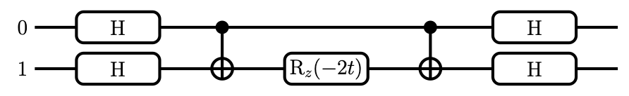
The Hadamard gates H rotate the qubits into the X basis, the CNOT prepares the parity and the
gate propagates under the XX interaction for time .
The parity-based algorithm does not introduce a reordering of spins on the qubits of the device. In general, on devices with a limited connectivity, additional SWAP gates need to be introduced to be able to run a circuit implementing the parity-based algorithm.
In the general case, the parity-based algorithm will lead to a larger gate count than a QSWAP algorithm. However, for devices with all-to-all connectivity (where each qubit can interact with every other qubit), inserting additional SWAP operations is not necessary. For those devices, the number of gates in the parity-based algorithm scales linearly with the number of XX, YY and ZZ operations in the Hamiltonian of interest.
Correlator Measurement
The spin correlator is measured in the time domain
where we have the total spin operators
which are the sum of the single-spin operators scaled by the gyromagnetic factors. In an infinite-temperature environment, the initial density matrix is . The correlator can be reconstructed by measuring the correlators , , , . Each of these is obtained as follows:
-
The qubits of the quantum computer are prepared in an eigenstate of the right operator , and the corresponding eigenvalue is stored.
-
This eigenstate is time-evolved with the trotterized algorithm, obtaining .
-
The expectation value of the left operator in the correlator is measured in this evolved state, obtaining for instance , given the left operator .
-
This procedure is either repeated for the full set of eigenstates of the right operator or sampled often enough that a representative trace is constructed as
With a growing number of spins, the number of basis states grows exponentially. To avoid this growth it is necessary to stochastically sample the initial states used in the calculation of the correlation function.
Basis choice in algorithms
It is convention to define the strong magnetic field in NMR along the Z-axis. However, the choice of the axis is arbitrary, as the fundamental problem is symmetric. When choosing to define the NMR system along the X-axis for example, the correlation functions that need to be calculated are and , but with respect to a transformed Hamiltonian, the single spin terms are terms. This transformation simplifies the construction of initial states in the quantum-computation.
To simplify this process, the HQS Qorrelator App allows the user to create quantum programs that use
the X-axis basis and automatically transforms Hamiltonians that are provided into the usual Z-axis
basis. The setting can be changed with the b_field_direction property of the NMRCorrelator
class, which is the main utility class of the HQS Qorrelator App.
Noise models
In the calculation of the NMR-correlation function a quantum algorithm is used to time-evolve a spin-Hamiltonian on a quantum computer. For quantum computers available presently, moderate noise occurs during the computation. This noise can however be interpreted as a coupling to an environment of the original NMR system.
The effect of the noise during the quantum computation is given by the noisy algorithm model. It maps incoherent noise during the execution of the algorithm to a continuous open system time evolution from the system. Calculating noisy algorithm model is a part of the HQS Qorrelator App and its theoretical basis is described shortly below. Its practical use is demonstarted in the examples.
For physical NMR systems, the environment seen by the spins is at infinite temperature. It is then desired that the noise during the quantum computation has an effect that is similar to an infinite temperature environment. The verification of this needs a detailed analysis of the noisy algorithm model. Such an analysis is provided by the HQS NMR tool. This thermalization analysis returns the essential information condensed to a simple quantity: the thermalization fidelity . Its value is defined to be between 0 and 1. The value means that the infinite-temperature environment interpretation is valid exactly, whereas numbers below 1, but well above 0, imply that this interpretation is approximatively valid. Values imply that the interpretation may not be valid. Different quantum algorithms lead to different thermalization fidelities .
Device noise
The effect of the noise during the quantum computation is modeled in our software by the noisy algorithm model. This adds noise to the classical simulation of the gate-based time propagation of the system state on quantum computer. Each gate comes with a noise that acts on qubits. The device can be set up with three different types of qubit noise:
- Damping
- Dephasing
- Depolarisation
The device initialization involves setting up independent rates of each decoherence channels (see the examples). To find out the noise probability corresponding to each gate, this is combined with the physical time needed to execute the gate.
In the modeling, we split each gate operation in an algorithm into the ideal unitary gate and a noise . Two simplest examples are
where and are superoperator representations of the unitary gate and the non-unitary noise. (In the superoperator representation the density matrix is a vector.)
The non-unitary noise gate is given by a Lindblad time-evolution over the physical gate time , , where is the Lindblad superoperator, defined below.
The Lindbladians are used to describe incoherent time evolution of the reduced density matrix of the qubits due to the effect of noise. We have . Damping of all qubits is described by
Here the spin operators act on the qubits. The dephasing noise corresponds to a Z (longitudinal) noise operator, The form is equivalent with the preceding Lindbladian, but we have used here . The depolarising noise is a sum of X, Y, and Z noise channels, with Lindbladian of the form For single-qubit systems this reduces to . Multiple Lindbladians can be added on the right-hand side of the density-matrix equation-of-motion, .
A fully thermalized state (having an equal probability of states and ) is a steady state of the depolarisation noise. It is also a steady state of dephasing noise, though dephasing does not necessary drive the system towards it, since it conserves the excitation number. However, with any addition of X noise or Y noise it does that. In contrast, the steady state of the damping noise is a state with no excitations, i.e., a pure state . It is then the magnitude of the damping noise that plays a central role in the full thermalization, as discussed below.
Effective noise
The thermalization analysis is done for the effective noise of the quantum algorithm. This is given by Lindbladian . This describes the collective effect of the noise gathered during the execution of the quantum algorithm. It is a Lindbladian acting on the spins of the NMR system. It is created as a sum of noise operations at each gate within one Trotter step. Each of these terms contribute via a Lindbladian of the original form, but with a unitary-transformed noise operator.
A minimal example is a two-gate Trotter step. Since gates are unitary and thereby invertible, we can write where and the effective noise operator is We see that when re-organizing the gates and noises to one overall gate plus noise construction, the first noise superoperator got transformed by . Equivalently, the original noise operator in the Lindbladian (such as ) got transformed by . Importantly, it turns out to be the superoperators and that define the effective Lindbladian. They map to a sum of individual noise Lindbladians, with noise operators (such as ) that have the transformed noise operators (such as ). In particular, the noise originating from dephasing or depolarisation is a summation of noise of unitary-transformed X,Y, or Z Pauli operators. This turns out to be important for the thermalization analysis, since such contributions can be mapped exactly to an environment at infintite temperature, as discussed below.
All noise contributions (over arbitrary many gates) within one Trotter circuit can be represented also in the general compact form Here we have also included contribution from the coherent gates as commutation with Hamiltonian , establishing the coherent time-evolution part. The operators are chosen such that they construct a full basis of superoperators. The software tool works in the basis of spin operators , i.e., Pauli matrices. This means that for us operators are either spin operators , or multiplications between different-site spin operators, .
The noise Lindbladian corresponding to the NMR quantum algorithm is calculated automatically by the HQS NMR tool. An example printing out the effective noise model is given in the practical examples.
Thermalization
The thermalization analysis is done for the effective noise, described by Lindbladian . The driving idea behind the following analysis is that in order to interpret the effective noise as an infinite temperature environment, it needs to drive the system to a fully mixed state. The fully mixed density matrix is proportional to the identity matrix, , where is the number of qubits, or equivalently spins.
Steady state of noise
We want that the fully thermalized system is a steady state of the system, . Since the mixed density matrix commutes with the Hamiltonian , this gives a condition
We first note that if there are no non-diagonal contributions, so that for , and if the operators are Pauli matrices or unitary tranformations of them, we will have , and the relation is valid. It follows that all contributions in the effective Lindbladian originating in the dephasing and depolarisation during the quantum algorithm satisfy this condition, since they contribute through summation of this type of terms. (Note that the collective summed representation of these terms in terms of operators can still have non-diagonal terms.) The thermalization analysis is then an analysis of the effective noise originating in the damping of the qubits.
Damping analysis
The software tool works in the basis of spin (Pauli) operators. We then continue by looking at the representation of the damping Lindbladian in this basis We observe that for damping noise On the other hand, for a combination of decay and excitation, we have If , we have . This noise can then be represented as a direct sum of X-noise Lindbladian and Y-noise Lindbladian. A fully-mixed density matrix is a steady state of such noise. It then corresponds to an infinite temperature environment.
On the other hand, we note that any single-qubit rotation of spins lead to combinations such as . For this and we have finite values of . However, . Also all common two-qubit gates do not lead to imaginary factors. We thus assign an imaginary part of to something that originates in damping.
According to these observations, we start constructing a definition of thermalization fidelity The contribution is calculated in the presence of all noise mechanisms (not just damping).
For pure damping the result is 0 whereas for a symmetric combination of damping and excitation (infinite temperature) the result is for any common single-qubit gate transformation of dephasing or depolarisation noise. For a finite damping, the presence of dephasing and depolarisation increases the fidelity, since they contribute only via the denominator (corresponding to the total decoherence rate).
Definition of thermalization fidelity
The above construction was done for damping in the Z basis. Generalizing to damping of all directions, and to arbitrary many spin sites, we now refine the definition to The index refers to that the numerator includes only single-spin operators as operators , such as . In the software, we use a factored approximation of the exact noise model, where higher-order noise operators are approximated by single-spin operators. This approximation includes only single-spin operators as the diagonals : the summation in the denominator is then done over all diagonal rates in the effective model.
The factoring approximation of the effective noise model can still include non-diagonal elements of type . These contributions can also cause deviations to the steady state in comparison to the fully mixed state, but with a smaller overall effect. A numerical analysis shows that the key terms stopping full thermalization come from terms of type , i.e., there is a matching spin index on two sides, associated with X and Y spin operators. According to this observation, we phenomenologically add a (second order) correction to the fidelity and finally define it as
It should be noted that we are neglecting a possible contribution from other higher-order contributions of type . To keep track of the size of dropped terms, we also define a discarded weight, which is a sum of the absolute values of the non-diagonal rates, divided by the overall rate, i.e., the above denominator.
Modeling physical noise
We consider incoherent errors as the predominant noise mechanism in quantum simulation. These errors can originate in interactions between qubits and a fluctuating environment. This mechanism influences the time evolution of the qubits in a way that the errors do not add up coherently. Simple examples of this are superconducting qubits coupled to lossy two-level systems, ion-trap devices with heated vibrational modes or unwanted control-pulse scattering, and spin-qubits in the presence of fluctuating background magnetic-field. During the last few decades, such noise mechanisms have been described successfully using the Lindblad master equation. The HQS Qorrelator App applies this method to model the effect of noise in a digital quantum simulation.
Master equation
Lindbladian
The noise mapping performed by the HQS Qorrelator App can be done for Markovian master equations. This means for noise mechanisms with short memory times. In particular, we apply master equations in the Lindbladian form:
where is the density matrix of the qubits (spins). Operators offer a basis for representing the noise operators, while matrix gives (generalized) noise rates. There is a freedom for definition of operators . So, only in combination with matrix (and particularly its non-diagonal entries) can we make judgements of the dominant noise processes and rates.
Noise operators
In our software, operators are chosen to be Pauli-matrices, (single-qubit noise on qubit ), and more generally Pauli products, (multi-qubit noise). An imaginary factor is added to Y-operators ( ) so that we avoid having imaginary numbers in matrix of the physical noise. (The effective rate matrix can however end up having imaginary entries.)
Rate matrix
For clarity in the following, we provide our definition of the spin-lowering and spin-raising operators:
The Lindblad equation for damping of qubit has the form:
Our noise matrix then has four non-zero values:
Similarly, dephasing of qubit 1 corresponds to noise matrix with non-zero entry:
Depolarisation corresponds to identical noise in all directions with rates:
This definition is based on the density matrix (here) approaching a diagonal matrix with rate .
Form of noise matrix for the physical model
Since our physical noise acts individually on each qubit , our physical noise matrix is a sum over individual contributions , where can be or . The matrix is real-valued. In the case where noise acts on all qubits at all times, the total noise matrix has the form:
whereas, if noise affects only qubits that are being operated on, we have:
It is important to note that this is the model for physical gates: the form of the effective noise can also include multi-qubit operators and imaginary (non-diagonal) rates, see the mapping section.
Noisy gates
Let us now introduce our model of gate-based quantum simulation with incoherent errors.
Super-operator matrix notation
For simplicity, we now use a notation where each noiseless gate operation (with a given unitary transformation ) is represented as matrix-multiplication:
On the right-hand side, the density “matrix” has become a vector, and the unitary transformations are matrices acting on it.
Model
In our modeling, we split each gate operation into the ideal unitary gate and non-unitary noise . We then replace each gate in some gate decomposition with:
where the noise transformation is given by the Lindblad time-evolution over some physical gate time ,
where is the Lindblad operator. Such a description can always be established if physical gate-times are much shorter than the decoherence rates related to this gate (). The question of how correct this description is of some specific hardware realization is then redirected to the question of the correct choice of noise matrix .
Foundations of noise mapping
On this page, we go through the mathematical foundations of the noise mapping performed by the HQS Qorrelator App. Physical noise on qubits transforms into effective noise on spins in the quantum simulation. For a detailed discussion, see the full paper on noise mapping.
Trotterization of time evolution operator
Decomposition blocks
Digital quantum simulation is based on Trotterization of the time-evolution operator, such that:
We consider a time-independent Hamiltonian and time-steps . The total Hamiltonian is divided into elements ,
which correspond to “small-angle” unitary transformations in the time evolution, .
The goal of the division is to have a sequence of unitary transformations which can be implemented efficiently on hardware.
An approximation (error) occurs when individual unitaries do not commute.
In the HQS Qorrelator App, such divisions are marked as circuit Decomposition_Blocks.
Small- and large-angle decompositions
Ideally, these unitaries can be implemented directly on hardware by the onset of single-qubit transitions or multi-qubit interactions, e.g., by control-field pulses. These operations then have one-to-one correspondence with equivalent small-angle gates,
As described in section modeling, in the presence of noise, each gate is assigned a noise operator .
However, some unitaries may need to be decomposed into a series of elementary gates,
Here, each gate comes with noise . In practice, such decompositions often include “large-angle” gates, such as CNOT gates or rotations.
Trotter error
The error in the simplest, first order, Trotter expansion is of size:
where , and is some typical energy of non-commuting terms in the Hamiltonian. Note that the error goes to zero in the limit .
Effective noise in the simulated system
Here, we detail how we map the physical noise of a quantum computer to effective noise in the simulated system. For this, it is enough to analyze unitary gates and non-unitary noise operations within one Trotter step. It also turns out that analysis of noise rotations can be done on each decomposition block separately.
Noise transformations
Let us first consider a decomposition of some unitary operation by two large-angle gates. The generalization to an arbitrary number of gates is straightforward.
By using the fact that gates are unitary, and thereby invertible, we can write:
where corresponds to a small-angle unitary,
and the effective noise operator is:
We see that the first noise operator got transformed by the (large-angle) unitary gate . Importantly, since both operators, and , describe small-angle (or probability) processes, these operators will later define the effective Lindbladian of the simulated system.
More generally, for an arbitrary decomposition we can write:
with:
It follows that the full time-evolution operator can be written as:
Here, each operator as well as is a “small-angle” (or probability) transformation. Finally, within the assumption that rotations over small-angle transformations can be neglected, we get the expression for the full Trotter step:
(It should be noted that the QSWAP algorithm of quantum simulation includes large-angle gates between decomposition blocks. The effect on the noise mapping, described above, is however analogous to state swaps and can be accounted for by simple “reordering dictionaries” in decomposition-block definitions.)
Lindbladian in the simulated system
Noise mapping is most intuitively formulated in terms of unitary transformations of Lindbladian operators. When constructing the effective model Lindbladian, we include all consecutive noise operations , each of them being some multiplication of transformed Lindbladians (see below), under one (exponentiated) Lindbladian,
Here, each summed Lindbladian has noise operators that are conjugated by the unitary gate defined by its corresponding decomposition, ,
(For native gates there will be no transformation, so that for these .) The final effective Lindbladian then takes the form:
with
and the anti-commutator
Here, an important noise scaling factor appears. We notice that the effective noise decreases with increasing Trotter time-step .
Error in the noise mapping
The above approximations are analogous to neglecting the Trotter error. First, we made the approximation that noise transformations can be restricted to individual decomposition blocks. The error of this approximation is of size:
where and are some typical Hamiltonian energy and noise probability of non-commuting elements between the two. Importantly, the error goes to zero in the limit .
Second, in the derivation of the Lindbladian, an error occurs when we combine consecutive noise terms (Lindbladians) under one exponent. This step has an error of size:
The validity of the noise mapping can be investigated numerically by comparing the solution for the original noisy circuit and for the effective Lindbladian.
Changelog
This changelog track changes to the HQS HQS Qorrelator App starting at version 0.2.0
0.11.1
- Fixed bug that was introducing an extra
right_operatorin the functionprepare_nmr_measurement_semi_spin_resolved. - Fixed the incorrect factor when computing the total correlator in the function
prepare_nmr_measurement_semi_spin_resolved.
0.11.0
- Removed
noise_placementoption. - Removed
optimization_leveloption and corresponding struct. - Switched from the
noise_modeoption toparallelization_blocks. This removes the option ofActiveQubitsOnlyfrom theNMRCorrelator, and the noise mode is changed by calling theparallelization_blocksoption, which takes a boolean input. By default, theNMRCorrelatoris initialized withAllQubitsas the noise mode (which can be changed toParallelizationBlocksby callingnoise_app.parallelization_blocks(true)). - Removed
readout_registeroption for the pyo3 interface of theInfiniteTemperatureCorrelator.
0.10.0
- Updated to new struqture 2.0 naming (Qubit -> Pauli).
- Switched from struqture 1.x output to 2.x output.
- Removed non-
_fixed_stepfunctions of theNMRCorrelator(includingspectrum_program) and of theInfiniteTemperatureWrapper. - Removed all initialisation options except for SumOverAllInitialStates.
- Updated docstrings to be more comprehensive.
- Removed
parallelfeature as it isn’t used anymore. - Added
trotter_timestepinput toInfiniteTemperatureWrapper.time_correlation_function.
0.9.0
- Updated minimum supported Python version to 3.9.
- Updated minimum supported Rust version to 1.76.
- Updated dependencies
0.8.3
- Removed old image for correlator measurements in the user documentation
- Added more tests.
- Updated Rust version and trimmed unused dependencies.
0.8.2
- Fixed an error in the documentation
0.8.1
- Fixed deploy issues
0.8.0
- Added support for inputs from struqture 2.0, and moved internal logic from struqture 1.x to 2.x
- Updated licensing package dependency that adds support for unknown entitlements
0.7.7
- Dependency updates to add support for new entitlements and to enable working with license file obtained by hqstage copy-license
0.7.6
- Improved license error messages.
- Improved documentation.
0.7.5
- Updated text of LICENSE_FOR_BINARY_DISTRIBUTION
0.7.4
- Dependency updates for fixing windows license checks
0.7.3
- Dependencies update to fix license checks on windows.
0.7.2
- Changed order of optimizations to enable fusion of Qsim operations when decomposition blocks are enabled
0.7.1
- Updated dependencies and removed prallel feature from default
0.7.0
- Add option to use decomposition blocks
- Add MultipleRotationGateSimplifier optimization from qonvert
0.6.1
- Update to dependency libraries with fix for license checks
0.6.0
- Refactoring functions not using fixed trotter timestep
0.5.0
- Added offline licensing checks
- Fix bug in the preprocessing of the Hamiltonian with field along X
0.4.1
- Add getters and setters for NMRCorrelator
- Refactored repository to include options for the direction of the magnetic field and processing of the Hamiltonian
- New user documentation
0.4.0
- Renamed the spin correlator app to the HQS Qorrelator App
0.3.0
- Update to dependency libraries
- Refactoring of code between App and dependency libraries
0.2.1
- Update to dependency libraries
0.2.0
- Fixed default number of measurements to be consistently 100_000