Quantum algorithm

We only describe the simplified algorithm for the infinite-temperature case implemented in the HQS Qorrelator App. For a detailed discussion of the standard correlation measurement we refer the reader to the literature.

Time evolution

To measure a correlation function in the time domain for a time difference \(t\), it is necessary to propagate the density matrix prepared on the quantum computer for a virtual time \(t\) (not to be confused with the time that passes in the laboratory frame of reference \(\tau\)).

The time propagation is handled with a standard Trotterization approach. The Hamiltonian of our NMR system can be written as a sum of partial Hamiltonians

\[ \hat H = \sum_k \hat H_k \]

and the time propagation under a partial Hamiltonian can be implemented on the quantum computer directly

\[ \hat U_k(t) = e^{- \textrm{i} \hat H_k t} \ . \]

For an NMR system, \(\hat H_k\) correspond to the onsite energy terms (Zeeman Hamiltonian) or the sum of all interaction terms between a specific pair of spins.

The time evolution under the full Hamiltonian can then be approximated as

\[ e^{-\textrm{i} \hat H t} \approx \prod_{\alpha=1}^{M} \prod_{k} \hat U_k\left(\frac{t}{M}\right) \ , \]

where the approximation is well controlled if \(M\) is sufficiently large.

The main difference in the methods provided by the HQS Software are

How each \(\hat U_k(t) \) is implemented in quantum gates.
How the necessary swapping of qubits between \( \hat U_k(t) \) is implemented.

The HQS software provides four optional algorithms:

QSWAP - The \(\hat U_k(t) \) involving two spins are implemented as gates that also swap the position of the two qubits. This algorithm uses the ParityBased algorithm for multi-qubit terms.
QSWAPMolmerSorensen - The QSWAP algorithm using variable angle Mølmer Sørensen XX interaction for multi-qubit terms.
ParityBased - The \(\hat U_k(t) \) involving two spins are implemented without swapping two spins with the help of two CNOT operations.
VariableMolmerSorensen The ParityBased algorithm using iable angle Mølmer Sørensen gates.

QSWAP

The QSWAP algorithm is the algorithm used by default. It implements every two-spin time propagation \(\hat U_k(t)\) with a so-called Qsim gate between neighbouring qubits (e.g. between \(0\) and \(1\) or \(2\) and \(3\) etc.). A Qsim gate applies the time evolution under a two-spin Hamiltonian

\[ \hat H = J_x \hat S^x_j \hat S^x_{j+1} + J_y \hat S^y_j \hat S^y_{j+1} + J_z \hat S^z_j \hat S^z_{j+1} \]

and also swaps the information content between the two involved qubits. Due to the repeated application of Qsim gates, the spins of NMR are swapped through the qubits in the quantum computer. At different stages of the algorithm, the same qubit can represent different spins. This "swap network" (for a Fermionic variant see Kivlichan et. al) also takes care of qubit routing. In many quantum computing devices, the number of other qubits a qubit can interact with is limited. For example, only next-neighbour interactions in 1D or 2D might be possible. For devices with at least 1D next-neighbour connectivity (meaning qubit \(0\) can interact with qubit \(1\), \(1\) with \(2\) and so on) the QSWAP algorithm already introduces all necessary SWAPS so that all gates in the produced quantum circuit can be applied without inserting additional SWAPS.

The QSWAP algorithm produces a Trotterization circuit with depth \(\mathcal{O}(N)\) and number of qubits \(\mathcal{O}(N^2)\), where N is the number of spins in the system.

Parity-Based

The parity-based algorithm directly implements the interaction between two qubits by applying a basis rotation, constructing the overall parity of the two qubits in one of the two qubits, and applying a single qubit rotation. For example, to implement an XX interaction, we can use the circuit

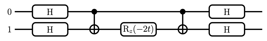
CNOT implementation of XX interaction

The Hadamard gates H rotate the qubits into the X basis, the CNOT prepares the parity and the \(\textrm{R}_z\) gate propagates under the XX interaction for time \(t\).

The parity-based algorithm does not introduce a reordering of spins on the qubits of the device. In general, on devices with a limited connectivity, additional SWAP gates need to be introduced to be able to run a circuit implementing the parity-based algorithm.

In the general case, the parity-based algorithm will lead to a larger gate count than a QSWAP algorithm. However, for devices with all-to-all connectivity (where each qubit can interact with every other qubit), inserting additional SWAP operations is not necessary. For those devices, the number of gates in the parity-based algorithm scales linearly with the number of XX, YY and ZZ operations in the Hamiltonian of interest.

Correlator Measurement

The spin correlator is measured in the time domain

\[ C(t) = \textrm{Tr}\left[ \hat{M}^{+}(t) \hat{M}^{-} \hat \rho_0 \right] \ , \]

where we have the total spin operators

\[ \hat{M}^{\pm} = \sum_j \gamma_j \hat S^{\pm}_j \ , \]

which are the sum of the single-spin operators scaled by the gyromagnetic factors. In an infinite-temperature environment, the initial density matrix is \( \hat \rho_0 = \frac{\hat 1}{2^N} \). The correlator \( \langle M^+(t)M^-(0) \rangle \) can be reconstructed by measuring the correlators \( \langle X(t) X(0) \rangle \), \( \langle Y(t) Y(0) \rangle \), \( \langle X(t) Y(0) \rangle \), \( \langle Y(t) X(0) \rangle \). Each of these is obtained as follows:

The qubits of the quantum computer are prepared in an eigenstate of the right operator \( m_n(0) \), and the corresponding eigenvalue \( m_n \) is stored.
This eigenstate \( m_n(0) \) is time-evolved with the trotterized algorithm, obtaining \( m_n(t) \).
The expectation value of the left operator in the correlator is measured in this evolved state, obtaining for instance \( \langle m_n(t) | X | m_n(t) \rangle \), given the left operator \(X\).
This procedure is either repeated for the full set of eigenstates of the right operator (currently the only available setting) or sampled often enough that a representative trace is constructed as

\[ \textrm{Tr}\left[ \hat{X}(t) \hat{Y} \hat \rho_0 \right] = \frac{1}{2^N} \sum_{m_n} m_n \langle X(t) \rangle_{m_n} . \]

With a growing number of spins, the number of basis states grows exponentially. To avoid this growth it is necessary to stochastically sample the initial states used in the calculation of the correlation function.

Basis choice in algorithms

It is convention to define the strong magnetic field in NMR along the Z-axis. However, the choice of the axis is arbitrary, as the fundamental problem is symmetric. When choosing to define the NMR system along the X-axis for example, the correlation functions that need to be calculated are \( \langle Y(t) Z(0) \rangle \) and \( \langle Z(t) Z(0) \rangle \), but with respect to a transformed Hamiltonian, the single spin terms are \(X\) terms. This transformation simplifies the construction of initial states in the quantum-computation.