Introduction
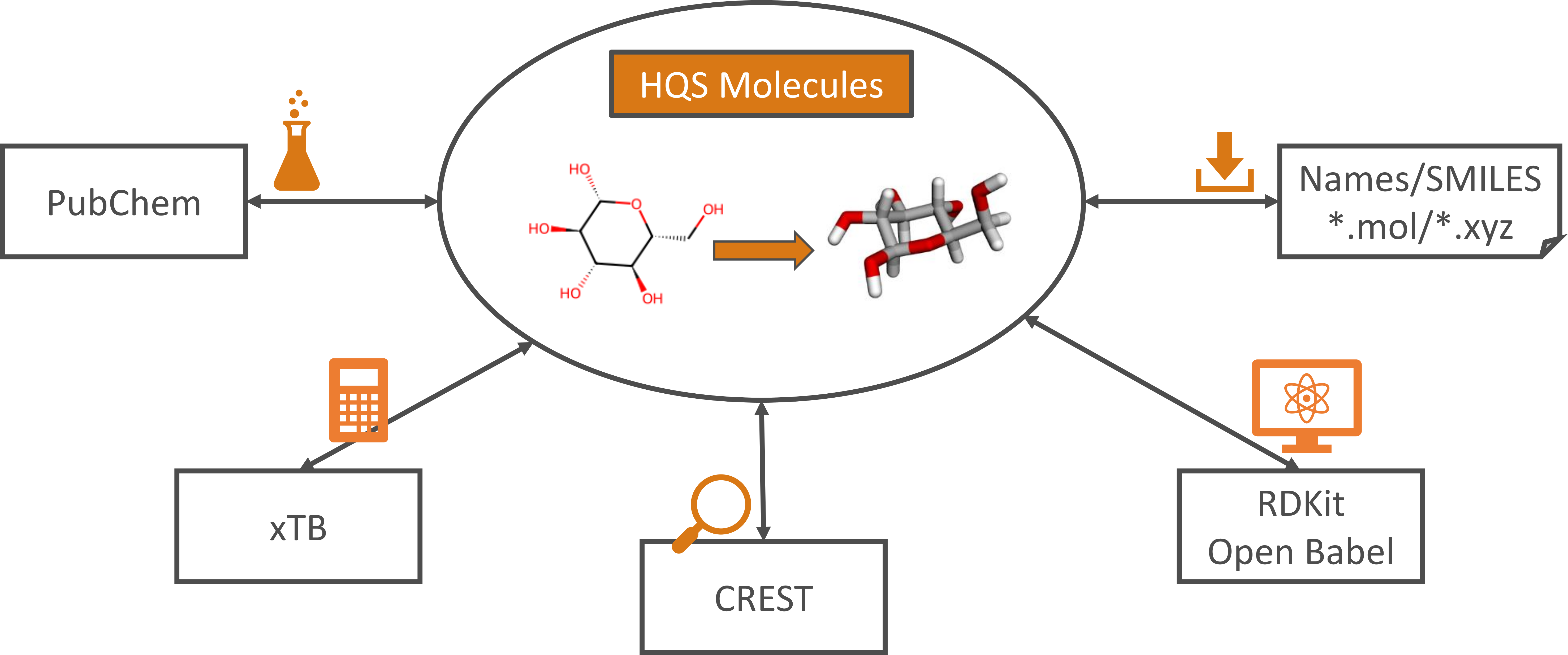
HQS Molecules is a user-friendly Python package designed to streamline computational chemistry workflows, with a focus on low-cost stages. Looking up a molecule name on PubChem, converting its SMILES string to an XYZ structure, optimizing its geometry and performing a conformer search: with HQS Molecules, all these steps take just a few lines of Python code. Wrappers around RDKit, Open Babel, xTB and CREST bundle these diverse open-source packages behind a uniform interface that is compliant with their respective licenses, while improving upon critical features. This makes HQS Molecules valuable both as a standalone tool for computational chemists, as well as a component in conjunction with other HQStage modules by HQS Quantum Simulations GmbH.
Features
HQS Molecules provides the following functionality to its users:
- Converting chemical structures from 2D to 3D representations. The RDKit and Open Babel packages are used to create XYZ structures from SMILES strings
or Molfiles, with an additional check for the correctness of the generated geometry. Standard chemistry literature and databases commonly encode molecules as representations of their 2D structural formula. On the other hand, 3D geometries are required to perform quantum-chemical calculations.
HQS Moleculesallows chemists and researchers in other fields to generate these conveniently and automatically. - API access to the PubChem database for name-to-structure and structure-to-name search. Direct access to the PubChem database via the Python API of
HQS Moleculesenables users to quickly retrieve a chemical structure by providing a compound name, or to search in reverse. This streamlines the process of gathering data for research and development, permitting automatization and reducing the potential for errors in manual searches.HQS Moleculescomplies with PubChem network access quotas and verifies that retrieved data is in the public domain. - Performing single-point energy calculations, geometry optimizations and frequency calculations with the semi-empirical xTB program.
HQS Moleculespermits users to integrate xTB functionality seamlessly into automated and efficient computational chemistry workflows with Python, enhancing productivity and enabling more complex simulations. - Performing conformer search through a Python interface for the CREST program with post-processing. Conformer search is essential for identifying the most stable molecular conformations and for understanding the conformational flexibility of molecules. By providing a Python interface,
HQS Moleculesmakes conformer search more accessible and easier to integrate into computational workflows. An additional refinement procedure for conformer ensembles has been developed exclusively withinHQS Molecules. Robustness and reliability is improved by reassigning conformers and rotamers, by carrying out a completion of the structural ensemble and by screening out transition states or other saddle points. - Reading and writing XYZ files. Being able to handle files with a single or with multiple geometries ensures compatibility with a wide range of computational chemistry tools and facilitates the exchange of molecular data between different software packages.
- Extensive usage of Pydantic to define input and output classes. Pydantic provides extensive functionality for data validation and serialization using Python type annotations. Besides ensuring correctness of data types, this permits input and output to be converted to and from JSON straightforwardly.
Example Use Cases
Generating three-dimensional structures, optimizing geometries, calculating molecular energies or vibration frequencies and sampling molecular conformations are crucial building blocks for molecular simulation workflows in the chemical pharmaceutical industries:
- Quantum chemistry calculations, with density functional theory (DFT) or with other methods, require three-dimensional geometries as their input. This information is rarely present in data sets that do not originate from a computational chemistry context.
HQSused features as implemented inHQS Moleculesto calculate thermodynamic properties of several thousand molecules for a customer with DFT: the starting point was a text file containing little more relevant information than compound names. - Whether you want to model chemical reactions or to calculate spectroscopic parameters:
HQS Moleculescan be used as part of your own Python-based workflow to provide the input for your favorite quantum chemistry software. Build upon the established expertise behind the open-source packages xTB, CREST, RDKit and Open Babel without needing to write your own interface. - Quantum computing algorithms for molecular electronic structure problems usually require a three-dimensional structure as an input, most often in XYZ format. Obtaining or creating this file can be a nuisance for specialists and non-specialists alike. With
HQS Molecules, a molecule name is all you need to generate three-dimensional geometries for a vast number of catalogued compounds. - The Active Space Finder is an open-source tool by
HQS Quantum Simulationsthat builds upon the PySCF software. It provides a user-friendly way to select active spaces for conventional multi-reference calculations and for quantum computing algorithms alike. UseHQS Moleculesto create input geometries for PySCF and the Active Space Finder.
Further Material
This manual contains extensive explanations on the usage of this module. In addition, please check the example notebooks for practical demonstrations of the utilities provided.
Installation
For general information on installing the module and downloading the example notebooks, please refer to the HQStage documentation.
Please note that
HQS Moleculesis currently only supported on Linux.
Parts of this module require third-party software packages that are not available for installation via pip: Open Babel, xTB and CREST.
The RDKit developers recommend installation via the conda-forge channel. Please note that the package on PyPI, which is installed by the
pipcommand, may not necessarily contain the latest released version.
Specific installation commands for an environment with the conda package manager are provided below.
-
Installation of
RDKit:
To make use of the latest version of the program, RDKit should be installed from the conda-forge channel. Installation via the PyPI server is also possible, but we have sometimes observed its versions being behind the releases on GitHub and on conda-forge. -
Installation of
Open Babel:
To benefit from the full scope of the 2D-to-3D structure conversion feature, we recommend installingOpen Babel. Open Babel can be obtained via the package managers of various Linux distributions (e.g.,apton Debian 12) or alternatively from the conda-forge channel. Note: 2D-to-3D structure conversion inHQS Moleculesuses the Open Babel package as a fallback option ifRDKitfails to generate a reasonable three-dimensional structure. It is possible to useHQS MoleculeswithoutOpen Babel, relying only onRDKitfor structure conversion. -
Installation of
xTB:
To make use of the interface to the xTB program for semiempirical calculations, thextbbinary must be provided by the user in thePATHvariable. We strongly recommend to download the binary release6.7.1from GitHub, since Hessian calculations with the GFN-FF method are known to fail with version6.7.0. Besides that, an installation fromconda-forgeis possible, in principle, but it is known to fail for specific calculations (like e.g. Hessian calculations for linear molecules). -
Installation of
CREST:
To make use of the interface to the CREST program for conformer search, thecrestbinary must be provided by the user in thePATHvariable. We recommend downloading the binary release3.0.2from GitHub.
Commands for the Installation of Third-Party Software
On Linux machines, we recommend working with a conda environment. It can be set up using distributions such as Anaconda, Miniforge or Mamba / Micromamba. The software packages mentioned above can be installed on Linux with the following commands:
# (1) Install Open Babel via apt
sudo apt install openbabel

# (2) Install RDKit in the current conda environment
conda install rdkit

# (3) Download and install the binaries of xTB
XTB_ARCHIVE="xtb-6.7.1-linux-x86_64.tar.xz"
XTB_URL="https://github.com/grimme-lab/xtb/releases/download/v6.7.1/${XTB_ARCHIVE}"
XTB_FOLDER="xtb-dist"
curl -LO ${XTB_URL}
tar -xvf ${XTB_ARCHIVE}
mv ${XTB_FOLDER} ${CONDA_PREFIX}/
ln -s ${CONDA_PREFIX}/${XTB_FOLDER}/bin/xtb ${CONDA_PREFIX}/bin/xtb
rm ${XTB_ARCHIVE}

# (4) Download and install the binaries of CREST
CREST_ARCHIVE="crest-intel-2023.1.0-ubuntu-latest.tar.xz"
CREST_URL="https://github.com/crest-lab/crest/releases/download/v3.0.2/${CREST_ARCHIVE}"
curl -LO ${CREST_URL}
tar -xvf ${CREST_ARCHIVE}
mv crest/crest ${CONDA_PREFIX}/bin/
rm ${CREST_ARCHIVE}
Molecular Name Lookup
HQS Molecules provides API access to the PubChem database, permitting name-to-structure and structure-to-name searches directly via Python scripts.
IMPORTANT: If you use the PubChem interface, data contained in the requests will be sent over the internet to the PubChem servers.
Name-to-Structure Search
Requests to PubChem are made via the PubChem data class, which stores the data retrieved after completion of each request. In the following example, a request is made using the molecule name:
from hqs_molecules import PubChem
pc = PubChem.from_name("2-methylprop-1-ene")
print(pc.name)
# Isobutylene
print(pc.cid)
# 8255
print(pc.formula)
# C4H8
print(pc.smiles)
# CC(=C)C
As shown above, the data retrieved is stored in the attributes
namefor the compound name,smilesfor the SMILES string,cidfor the PubChem compound ID, andformulafor the molecular formula (as aMolecularFormulaobject).
Note: the name stored in the name attribute may differ from the argument supplied for the request: the most entries for a compound on PubChem list multiple synonymous names, but the name attribute contains the representative title name selected on PubChem. This is illustrated in the example below:
from hqs_molecules import PubChem
pc = PubChem.from_name("acetylsalicylic acid")
print(pc.name)
# Aspirin
Structure-to-Name Search
Likewise, a reverse search can be performed using a SMILES string:
pc = PubChem.from_smiles("COC1=C(C=CC(=C1)C=O)O")
print(pc.name)
# Vanillin
Search by PubChem Compound Identifier
Finally, requests can be made using the PubChem compound identifier:
pc = PubChem.from_cid(145742)
print(pc.name)
# Proline
print(pc.smiles)
# C1C[C@H](NC1)C(=O)O
An important feature of the PubChem class is that it verifies the depositor of individual data items retrieved. Data is only made available if PubChem is listed as the data source.
As shown in the section on 2D to 3D structure conversion, a SMILES string can be used to generate a three-dimensional representation.
Structure Conversion
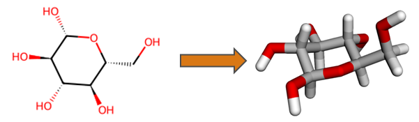
An important feature of HQS Molecules is conversion of two-dimensional molecular structural formulas into three-dimensional geometries, as exemplified below for the glucose molecule. Functionality of RDKit and Open Babel is built upon in order to obtain results more reliably than with either software on its own. Generated three-dimensional structures are verified against the input, increasing trustworthiness for automated workflows.
Simple 2D to 3D Conversion
Input: SMILES strings and Molfiles are supported as input for the functions smiles_to_molecule and molfile_to_molecule, respectively.
Output: Both functions return a Molecule object containing three-dimensional atomic coordinates. In addition, the returned object contains the overall molecular charge, which is always included in a Molfile or a SMILES string. The spin multiplicity field is set to None, as it cannot be derived unambiguously from the input.
The structure conversion employs the respective feature of RDKit as its first choice, and uses Open Babel as a backup in case that structure conversion with RDKit fails. After generating a three-dimensional structure, a bonding graph is determined using distance criteria and used to verify the generated structure against the input. If the composition and the bonding graphs do not match, then the structure is rejected.
Having the SMILES string of a molecule at hand, it is straightforward to create its 3D representation with a function call. For example, we may first obtain the SMILES string of a molecule from PubChem:
from hqs_molecules import PubChem, smiles_to_molecule
pc = PubChem.from_name("propane")
print(pc.smiles)
# CCC
The three-dimensional structure is created from the string with a call to smiles_to_molecule:
mol = smiles_to_molecule("CCC")
Conversion of a structural formula stored in a Molfile ("my_molecule.mol" in this example) proceeds similarly:
from hqs_molecules import molfile_to_molecule
mol = molfile_to_molecule("my_molecule.mol")
An optional check can be carried out with either of the conversion functions by supplying a molecular formula as an argument. The conversion fails if the input does not match the provided formula. In that case, the formula needs to be represented as a MolecularFormula object.
from hqs_molecules import MolecularFormula, PubChem, smiles_to_molecule
pc = PubChem.from_name("propane")
# succeeds
mol = smiles_to_molecule(pc.smiles, formula=pc.formula)
# raises an exception
mol = smiles_to_molecule(pc.smiles, formula=MolecularFormula.from_str("C3H7-"))
The code above will raise an error in the last line since a wrong formula of propane is provided.
Utilities for RDKit
The HQS Molecules module includes convenience functions to create RDKit Mol objects from SMILES strings, Molfiles, or XYZ files. These objects represent molecular information within the RDKit package.
Both the smiles_to_rdkit and molfile_to_rdkit functions accept an argument addHs. By default, it is set to True, causing explicit hydrogen atoms to be added in the generated object. Setting addHs = False suppresses the addition of explicit hydrogens; only hydrogens that were already explicitly represented within a Molfile are retained.
from hqs_molecules import smiles_to_rdkit
# The object generated contains 11 atoms.
rdkit_mol = smiles_to_rdkit("CCC")
# The object generated contains 3 atoms.
rdkit_mol = smiles_to_rdkit("CCC", addHs=False)
When creating an RDKit Mol object from an XYZ file, this option does not apply as the hydrogen atoms always have to be represented explicitly. However, the xyzfile_to_rdkit function accepts another important argument (apart from the XYZ file name or path) which is the charge. This argument is necessary to specify the total net charge of the molecule in order to find the correct atomic connectivity and it is set to 0 by default for convenience. Since an XYZ file does not contain any information about chemical bonds by itself, this evaluation is done inside the xyzfile_to_rdkit function using RDKit.
For the following example, assume we have two valid XYZ files called benzene.xyz with the three-dimensional structure of a benzene molecule and nh4.xyz with the structure of an ammonium cation.
from hqs_molecules import xyzfile_to_rdkit
# The object generated contains 12 atoms, 6 single bonds, and 6 aromatic bonds.
rdkit_mol = xyzfile_to_rdkit("benzene.xyz")
# This will raise a `ValueError`
rdkit_mol = xyzfile_to_rdkit("nh4.xyz")
# This works and the object generated contains 5 atoms and 4 single bonds.
rdkit_mol = xyzfile_to_rdkit("nh4.xyz", charge=1)
Other Functionalities
Apart from converting different types of input such as SMILES strings or Molfiles to molecule objects,
the structure_conversion submodule provides functions to the opposite and convert molecule objects, XYZ files or Molfiles (or their contents) to SMILES strings.
from hqs_molecules import xyz
from hqs_molecules.structure_conversion import molecule_to_smiles, smiles_to_molecule

smiles = "C1=NC2=NC=NC(=C2N1)N"  # adenine
mol = smiles_to_molecule(smiles)
print(molecule_to_smiles(mol))  # "Nc1ncnc2nc[nH]c12"
Be aware that the input SMILES string is not necessarily the same as the one returned by the functions as there are usually many ways to represent the same molecule as a SMILES string. The one returned by default is the canonical and isomeric one according to RDKit.
Expert Usage
Features described in the remainder of this section are only intended for expert usage.
An RDKit Mol object can be converted to a three-dimensional structure by passing it to the function rdkit_to_molecule. It is a low-level function that calls RDKit without resorting to Open Babel as a backup. Nonetheless, it performs a consistency check for the generated structure. If the RDKit Mol object was created without the addition of explicit hydrogens (addHs = False), this conversion may fail due to a composition mismatch.
The low-level functions to perform structure conversion using only Open Babel are available via smiles_to_molecule_obabel and molfile_to_molecule_obabel. These functions require a SMILES string or a Molfile as their input, respectively. A separate consistency check of the generated structure is also performed here.
XYZ File Handling
HQS Molecules provides a module to read and write XYZ files.
The XYZ format is very commonly used to represent the spatial arrangement of atoms in a molecule.
Being able to read and write these files ensures compatibility with a wide range of computational chemistry tools and facilitates the exchange of molecular data between different software packages.
Reading and Writing XYZ Files
XYZ files are read using the function xyz.read. It can be called either with a Path object or a
string representing a file path; alternatively, it may be provided with a file-like object.
from hqs_molecules import xyz
# providing a file name
molgeom = xyz.read("molecule.xyz")
# providing a file-like object
with open("molecule.xyz", "r") as f:
    molgeom = xyz.read(f)
XYZ files contain atomic positions and chemical element symbols, but no information on charge and spin multiplicity. Therefore, the function returns a MolecularGeometry object with element symbols and atomic positions. It can be easily converted to a Molecule object by providing information on the charge and, optionally, on the multiplicity:
mol = molgeom.to_molecule(charge=0)
mol = molgeom.to_molecule(charge=0, multiplicity=1)
XYZ files can be written to disk using the function xyz.write by providing either a MolecularGeometry or a Molecule object (the latter is a subclass of the former). The function can either create a file at the specified path, or write to a file-like object.
Converting Strings with XYZ Information
In some cases, the content of an XYZ file may be present in a string, or may need to be converted to a string. Such cases can be handled generally using the aforementioned functions xyz.read and xyz.write operating on a io.StringIO object (instead of a Path object or a string). However, the HQS Molecules module also provides convenience functions xyz.parse_string and xyz.get_string that read and format strings with XYZ content directly:
# creates a string from a MolecularGeometry or Molecule object
s = xyz.get_string(mol)
# creates a MolecularGeometry object from a string with XYZ content
molgeom = xyz.parse_string(s)
The xyz.get_string method takes a second, optional argument comment to write a single-line string into the comment line of the XYZ file.
Working with Comments in XYZ Files
The XYZ file format permits one single line with an arbitrary comment inside a molecular geometry definition. Some programs use this comment line to store specific information. When importing an XYZ file in HQS Molecules the comment can be requested by setting the argument return_comment to True. This causes the function to return a tuple with the molecular geometry and the comment line.
from hqs_molecules import xyz
molgeom, comment = xyz.read("molecule.xyz", return_comment=True)
Likewise, a comment line can be exported to an XYZ file by providing it in the comment argument.
xyz.write("output.xyz", molgeom, comment="comment line ...")
Information on charge and spin multiplicity can be written into the comment line of an XYZ file using the function xyz.write_with_info. Unlike the read and write functions, it requires a Molecule object, as the MolecularGeometry class lacks information on charge and multiplicity.
XYZ Trajectory Files
Trajectories may be stored in XYZ files simply by concatenating XYZ geometries. Such files can be read using the function xyz.read_geometries. File paths (represented by a Path object or a string) as well as file-like objects are supported as its input argument. By default, the function returns a list of molecular geometries. Setting return_comments to True causes it to return a list of tuples instead, each tuple containing a geometry and its associated comment.
# Returns an object of type list[MolecularGeometry]
geom_list = xyz.read_geometries("trajectory.xyz")
# Returns an object of type list[tuple[MolecularGeometry, str]]
tuple_list = xyz.read_geometries("trajectory.xyz", return_comments=True)
In order to write a trajectory file, the function xyz.write is used (as for individual geometries), but with a list of geometries instead of an individual geometry.
xyz.write("output.xyz", geom_list)
If individual comments need to be provided for each geometry, this is best done by working with a file stream, as shown in the example below:
with open("output.xyz", "w") as f:
    for step, geometry in enumerate(geom_list):
        xyz.write(f, geometry, comment=f"step number {step}")
If an object of type Trajectory is provided to the function xyz.write_with_info, then the energies for each step, along with charge and multiplicity, are written into the comment lines of the trajectory file.
Semi-empirical Calculations with xTB
This HQS Molecules module contains a Python interface to perform calculations with the xTB software package.
The xTB (extended tight binding) program package is developed by the research group of Prof. Stefan Grimme at the University of Bonn. It contains implementations of the semi-empirical quantum-mechanical methods GFNn-xTB (n = 0–2) as well as of the GFN-FF force field ("GFN" stands for Geometries, Frequencies, and Non-covalent interactions, for which it has been parametrized).
It uses shared-memory OpenMP parallelization, controlled for instance via the OMP_NUM_THREADS environment variable.
For more details, see the manual.
HQS Molecules interfaces the following features, permitting them to be used conveniently from within Python workflows:
- Single-point energy calculations,
- Structure optimizations,
- Gradient calculations,
- Frequency calculations,
- Stable optimizations including Hessian calculations, and the
- Biased Hessian.
Single-point energy calculations
The energy of any meaningful set of atomic coordinates with a specific charge and multiplicity
can be calculated using the single_point function. Calculations are performed with the GFN2-xTB method by default, or alternatively with the GFN-FF method.
Input
The first mandatory argument of the function is a Molecule object, as the charge and multiplicity need to be known to perform a calculation.
Note: the functions for reading an XYZ file return MolecularGeometry objects, which contain neither charge nor spin information. A MolecularGeometry objects can be easily converted to a Molecule object by providing information on the charge and, optionally, on the multiplicity, as described in the XYZ File Handling chapter. On the other hand, the 2D-to-3D structure conversion functions return Molecule objects with charge but without spin information.
Keyword arguments for single-point energy calculations
Calculation settings can be adjusted with the following keyword arguments:
force_field: Use GFN-FF force-field (defaults toFalse, in which case the GFN2-xTB method is used).solvent: By default, calculations are performed in vacuum. If the name of a solvent is provided, the implicit solvation model ALPB (analytical linearized Poisson-Boltzmann) will be used in the calculation.create_tmpdir: Run the calculation in a temporary folder that is deleted with completion of the calculation (the default is set toTrue).
Output
The single_point function returns a float with the single-point energy in Hartree.
If an implicit solvation model is used, the solvation contribution ("Gsolv" in the xTB output) is
part of the single-point energy.
Example
An example is provided here:
from hqs_molecules.xtb import single_point

energy = single_point(molecule, force_field=False)
Solvents
HQS Molecules supports using the ALPB implicit solvation model implemented in the xTB code. By default, calculations are performed in vacuum. Parameters of specific solvents can be selected by providing the solvent name as a string to the solvent keyword argument of the various wrapper functions, such as solvent="Water".
The following loop prints all solvent names that have been defined in the interface:
from hqs_molecules import xtb
for name, keyword in xtb.SOLVENT_KEYWORDS.items():
    print(f"{name:20}:  {keyword}")
It is possible to specify keys or values of the xtb.SOLVENT_KEYWORDS dictionary, so that
"Octanol (wet)" or "woctanol" are equally valid. In addition, the input is treated
case-insensitively.
For more information on defined solvents, please check the section in the xTB manual.
Example on specifying a solvent in a single-point energy calculation:
from hqs_molecules.xtb import single_point

energy = single_point(molecule, solvent="Water", force_field=False)
Structure optimization
xTB can optimize atomic positions in a molecular system to find a nearby local minimum of the
total energy representing an equilibrium structure.
This feature is embedded into HQS Molecules through the optimization function.
Keyword arguments for geometry optimizations
In addition to the arguments for single-point energy calculations, the following options are available:
-
opt_levelwith different optimization accuracy settings as defined by xTB. Possible values for this option are defined in thextb.OptLevelEnum. By default, the very tight criterion is employed (OptLevel.VTight), whereas the xTB software itself usesOptLevel.Normal. For the definition of the options, ordered from low to high accuracy below, please refer to the xTB documentation:- Crude
- Sloppy
- Loose
- Lax
- Normal
- Tight
- VTight
- Extreme
-
max_cyclesis the maximum number of optimization iterations. By default, it is set toNone, which means thatmax_cyclesis automatically determined by the xTB software depending on the size of the molecule (check above link).
Output
Calls to the optimization function return a Trajectory object containing the optimization trajectory (Trajectory.structures) as a list of Molecule objects and the energies (in Hartree) for each step (Trajectory.energies) as a list of floats.
Most of the time, the quantities of interest are the optimized geometry and its energy. To access these, a Trajectory object contains two types of attributes: Trajectory.last and Trajectory.last_energy contain the last geometry and its energy, respectively; Trajectory.lowest_energy and Trajectory.lowest contain the lowest energy and the corresponding geometry. Trajectory.lowest_step returns the index of the energetically lowest geometry. In many cases, the last step may also be the one with the lowest energy.
Note that the energy might increase slightly at the end of an optimization (within the given tolerance criteria) or it can converge to saddle point, in which case the lowest-energy geometry can be the anywhere along the trajectory, even at its beginning.
The trajectory can be written to an XYZ file using the write or write_with_info (includes energies) functions of the xyz module.
Example
The following box illustrates some general ideas behind executing a geometry optimization, starting from a Molecule object.
from hqs_molecules import xyz
from hqs_molecules.xtb import optimization

# perform optimization
opt_data = optimization(molecule, solvent="water")

# Write the trajectory into an XYZ file
xyz.write_with_info(file="trajectory.xyz", mol=opt_data)

# Optimized structure: here it is assumed to be in the last step.
opt_molecule = opt_data.last  # Molecule object
opt_energy = opt_data.last_energy  # float
Gradient calculation
The nuclear gradient (first derivative of the energy with respect to the atomic coordinates) is calculated at each step of an optimization procedure. An optimization is converged if the energy no longer changes and the (norm of the) gradient is close to zero.
A single-point gradient can be calculated using the gradient function with the same arguments as a single_point procedure. It returns a nested list of floating point numbers, representing an N × 3 matrix (where N is the number of atoms in the molecule). Each value in the list corresponds to the derivative of an atomic position with respect to the x, y or z coordinates, represented in units of Hartree Bohr−1.
Vibrational frequency calculations
The Hessian matrix (a matrix of second derivatives of the energy with respect to the atomic coordinates) is used to determine the nature of a stationary point, vibrational frequencies, molecular vibrational spectra, and thermochemical properties.
In xTB, the Hessian matrix is calculated semi-numerically, i.e., from the analytical gradient using finite differences.
HQS Molecules provides the frequencies wrapper function to calculate vibrational frequencies and thermochemical corrections.
Keyword arguments for vibrational frequency calculations
In addition to the options for single-point energy calculations, this function also accepts a temperature argument. This allows the user to define the absolute temperature for the calculation of thermochemical corrections. By default, the calculation will be performed at 298.15 K, but any other non-negative temperature can also be specified.
Nature of the input geometry
When calculating vibrational frequencies for a stationary point (an optimized equilibrium structure or a saddle point), it is important to use the same method for the frequencies as for the preceding geometry optimization; the potential energy surfaces of different methods have stationary points at different geometries.
Frequency calculations are often used to ascertain if a stationary point is a minimum or a saddle point. A molecule of N atoms has 3N degrees of freedom: three translational degrees, three rotational degrees (two for linear molecules), and 3N − 6 vibrational degrees (or 3N − 5 for linear molecules). For a minimum, the frequencies associated to those vibrational degrees need to be positive; for a transition state (i.e., a first-order saddle point), exactly one of them needs to be imaginary.
Output
The return value is a tuple with a VibrationalAnalysis and a Thermochemistry object.
VibrationalAnalysis objects contain vibrational frequencies and normal modes in their fields and properties:
modes: a list ofVibrationalModeobjects, which contain the vibrationalfrequency(in cm−1), the infrared (IR) intensity (ir_intensityin km mol−1) as well as the Cartesiandisplacementsof the normal mode as attributes.frequencies: a list with the vibrational frequencies (in cm−1) in strictly increasing order. This list contains 3N − 6 elements (or 3N − 5 for linear molecules). By convention, imaginary frequencies are represented as negative numbers.hessian: nested lists representing a 3N × 3N matrix with the nuclear Hessian (in Hartree Bohr−2).reduced_masses: a list with the reduced masses (in atomic mass units) associated with the normal modes.ir_intensities: a list with the IR intensities (in km mol−1) containing 3N − 6 or 3N − 5 elements.displacements: a list with the Cartesian displacements for each normal mode that are normalized to unity.is_linear: a property flag indicating whether the molecule is linear or not.natoms: the number of atoms in the system, inferred from the dimensions of the displacements.
Thermochemistry objects contain thermodynamic data calculated with the modified rigid rotor and harmonic oscillator (mRRHO) approximation.
The following data is accessible:
temperature: the temperature (in K) used to calculate the thermodynamic properties.energy: the total electronic single-point energy (in Hartree)enthalpy: the enthalpy (in Hartree), including the total electronic energy.entropy: the entropy (in Hartree K-1).gibbs_energy: the Gibbs energy (in Hartree) as a property. It not stored explicitly, but calculated from the enthalpy, entropy and temperature in the object. Like the enthalpy, it includes the total electronic energy.
When using an implicit solvation model, the xTB code calculates a solvation contribution,
labelled as "Gsolv" in the output of the xTB binary.
Even though "Gsolv" is technically a free energy contribution, it is reported as part of the total
electronic energy by the xTB code.
Therefore, the solvation contribution is also part of energy in the Thermochemistry object
returned after a Hessian calculation with the xtb module.
Example
from hqs_molecules.xtb import frequencies

vib_analysis, thermochem = frequencies(opt_molecule, temperature=100, solvent="water")

print("Single point energy:", thermochem.energy)
print("Frequencies:", vib_analysis.frequencies)
print(
    f"At {thermochem.temperature} K, "
    f"the enthalpy is {thermochem.enthalpy} Eh, "
    f"the entropy is {thermochem.entropy} Eh/K, and "
    f"the Gibbs energy is {thermochem.gibbs_energy} Eh"
)
Stable optimization: calculating equilibrium structures reliably
With a simple geometry optimization, there is no guarantee to obtain a minimum on the potential energy surface; a converged structure can also be a saddle point. Vibrational frequencies need to be calculated for a full characterization. Only if all of them are non-negative, a minimum has been found.
If imaginary frequencies are found, a displacement along the associated normal mode is a good starting point for a new optimization. In difficult cases, optimizations followed by frequency calculations may need to be repeated multiple times in order to find a genuine local minimum.
Such a composite calculation is provided by HQS Molecules with the opt_with_hess function. It repeats the Hessian and optimization calculations until no imaginary frequencies are found. If the maximum number of restarts (indicated by the max_restarts keyword, 4 by default) is reached without converging to a minimum, an exception is raised by default.
The latter behavior can be altered by setting fail_with_saddle to False, in which case the non-converged trajectory is returned together
with the Hessian result from the lowest-energy structure. The latter can be obtained from the lowest property
and can be used for a successive calculation.
Note that the restart geometries used in opt_with_hess are generated by the xTB code upon encountering a saddle point in a Hessian calculation. These are suited to displace the geometry away from a saddle point. As there is no control over the direction along a normal mode with imaginary frequency, the feature is meant to converge to a nearby local minimum, but not for a systematic exploration of reaction paths.
Input
Since the function combines optimizations with frequencies, it requires the same arguments as the optimization function, with an option to provide a temperature argument (for the thermodynamic properties) and max_restarts.
Output
The return value is a tuple containing a Trajectory object (as for an optimization), and
VibrationalAnalysis and Thermochemistry objects (as for a frequency calculation). The trajectory concatenates the geometries and energies of all optimizations performed within the procedure. On the other hand, the VibrationalAnalysis and Thermochemistry objects contains information for the converged geometry, determined by the overall lowest energy.
If fail_with_saddle is set to False, the appropriate results for the lowest-energy structure are returned, even if it could not be converged to a stable minimum.
Example
A simple call to this procedure can be made as exemplified below:
from hqs_molecules import xtb, xyz
molecule = xyz.read("input_geometry.xyz").to_molecule(charge=0, multiplicity=1)
trajectory, vib_analysis, thermochem = xtb.opt_with_hess(molecule)
Biased Hessian
Hessian calculations for vibrational frequencies or thermochemical contributions are normally performed at stationary points of the potential energy surface. Therefore, the geometry optimization and the Hessian calculation need to be performed with the same method.
However, Spicher and Grimme proposed a method ("single-point Hessian") to calculate the Hessian for stationary points that were optimized with a different method. Therefore, the geometry can be optimized with a more expensive method, while xTB is used to obtain a quantity resembling the Hessian. In a nutshell, it employs the following steps:
- The input structure is re-optimized under application of a biasing potential, which constrains the atoms to remain close to their original positions.
- The Hessian is calculated at the new, slightly distorted geometry under the application of the biasing potential.
- Finally, the frequencies are re-scaled to reduce the impact of the biasing potential.
HQS Moleculesprovides the function biased_hessian to interface the described method in the xTB package. Its usage is analogous to the function frequencies described above.
Conformer and Rotamer Search
Many molecules, especially in organic chemistry, have a large degree of conformational freedom. At relevant temperatures, they are not represented by a single minimum on the potential energy surface, but rather by an equilibrium between rapidly interconverting minimum structures. Thus, comparing experimental measurements with theoretical data often requires consideration not only of a single structure, but of an entire thermodynamically accessible conformational ensemble.
CREST (Conformer–Rotamer Ensemble Sampling Tool) is a program used to perform conformer searches
using the methods implemented in the xTB package.
The wrapper function find_conformers provided by HQS Molecules interfaces CREST (which uses xTB as its engine)
to search for low-energy conformers and rotamers of a given molecule.
HQS Molecules reads the number of parallel CPU threads from the OMP_NUM_THREADS environment variable and passes the value on as the number of parallel threads to be used by CREST. If unspecified, the number defaults to 1. Note that this is different from the behavior of the CREST binary itself, which does not check OMP_NUM_THREADS, but requires the degree of parallelism to be specified through a commend-line argument.
HQS Molecules implements a refinement procedure that is described in this section. It improves the completeness and consistency of conformer search results, which is vital for applications such as NMR parameter prediction.
Conformers and Rotamers
Conformers are distinct minima on the potential energy surface that are separated by sufficiently low barriers, such that they can interconvert at a given temperature. Often, this occurs through torsions around single bonds.
The concept of conformers can be generalized to structures that are not minima, such as transition states or constrained minima. These sets of related structures connected by low barriers are referred to as conformations.
In our context, rotamers are defined as interconverting structures that can be represented as permutations of the atoms in a conformer. A simple example of rotamers are the structures related by the rotation of a methyl group (–CH3) in an organic molecule. Somewhat less intuitively, the two chair structures of cyclohexane are also regarded as rotamers, as their structures can be superimposed. This definition was introduced by Grimme and co-workers in the context of automated NMR calculation, and differs from the definition of rotamers by IUPAC. See also the publication on the CREST software by Pracht and co-workers.
Input
The find_conformers wrapper function performs three successive steps:
- Conformer/rotamer ensemble search using CREST.
- Reassignment of the structural ensemble and completion of the rotamer sets using a procedure developed within
HQS Molecules. - Calculation of vibrational frequencies and discarding structures corresponding to saddle points.
It employs the following arguments:
molecule: mandatory specification of the input molecule as aMoleculeobject.solvent: optional specification of the solvent as a string. By default, the calculation is performed in vacuum. Please refer to the xTB section for more information.create_tmpdir: set toTrueby default, so that the calculation is performed in a temporary directory that is deleted upon finishing the calculation.force_field: it is set toTrueby default; set toFalseto perform the conformer search with GFN2-xTB instead.freq_threshold: the frequency threshold in cm−1 below which conformers are considered saddle points and thus discarded.ignore_enantiomorphism: it is set toFalseby default, such that mirror images are considered to be different structures and not equivalent rotamers.similarity_tolerances: the numerical tolerances for bond distances, bond angles, and dihedral angles for structures to be identified as equivalent.do_rotamer_completion: it is set toTrueby default, to enable completion of rotamer sets through permutational logic.temperature: the absolute temperature in K used for predicting thermodynamic properties (such as the Gibbs energy) in the frequency calculations.
The argument similarity_tolerances is of type SimilarityTolerances, which is a data class containing default values for the absolute and relative tolerances
for bond distances, bond angles, and dihedral angles to be considered equivalent in the structure-matching procedure.
Please note that bond and dihedral angles are compared via the absolute value of the complex exponential of the respective angle difference,
and the tolerances refer to those values.
It is important to emphasize that the function uses GFN-FF by default to reduce computational code. In contrast, the wrapper functions for the xTB package use GFN2-xTB by default.
Algorithm
Different workflows have been implemented for CREST over the years. It is worth noting that find_conformers calls CREST with the static metadynamics simulations algorithm, instead of the computationally less demanding extensive metadynamic sampling utility that is the default when running CREST directly.
Note also that the grouping of conformer and rotamer structures as determined in the CREST calculation is ignored, and all the structures are regrouped by our own procedure as follows:
-
First, a plain list of structures is generated from all conformers and rotamers obtained from CREST.
-
Then, the structures are all compared among each other, grouping them by conformers purely based on their 3D structural parameters (bond lengths, bond angles, and dihedral angles).
-
If they are the same within a given numerical threshold, they are considered to be equivalent structures (rotamers), and the atomic mapping (or permutation) relative to the representative conformer is stored for each of the rotamers instead of all the geometries themselves.
-
Successively, the set of rotamer mappings is checked for completeness by multiplying all permutation matrices and verifying if the result is already present in the set of permutations. That way, a full set of rotamers is determined for each conformer as long as the initial set of structures is sufficiently representative.
-
As a last step of the procedure, structures corresponding to energetic saddle points are discarded.
Output
The output is an instance of the ConformerEnsemble class.
-
Important methods of the class provide access to flat lists of all conformer structures and energies (
get_conformer_structures,get_conformer_energies), -
as well as the number of rotamers per conformer (
get_degeneracies). -
Detailed information on conformers with their individual rotamers is contained in the items of the
conformerslist. Each element of this list is of theConformertype.- Apart from having the
structure - and
energyattributes, - it also has a list of
atom_mappingsdictionaries, which represent the atom permutations of the referencestructureto the different rotamers.
- Apart from having the
Note that the outcome of calculations performed with CREST directly may differ somewhat between runs repeated under identical conditions. Moreover, the starting geometry affects the conformer search. The refinement steps described above substantially increase the consistency of the conformer search results.
Example
An example of a conformer/rotamer search, starting from a molecule name:
from hqs_molecules import PubChem, find_conformers, smiles_to_molecule

pc = PubChem.from_name("1-butene")
molecule = smiles_to_molecule(pc.smiles)
conf_data = find_conformers(molecule)

print(f"Found {len(conf_data)} distinct conformers.")  # or conf_data.num_conformers
# Found 3 distinct conformers.
print(f"Conformer 0 has {conf_data.get_degeneracies()[0]} rotamers.")
# Conformer 0 has 3 rotamers.
Important Data Structures
This section provides a short description of important data structures used for input and output
in functions provided by HQS Molecules. Many of these classes are implemented as Pydantic models. Pydantic provides data validation and parsing using Python type annotations. By leveraging Pydantic, the package ensures that input and output data are correctly formatted and validated, reducing the likelihood of errors and improving the robustness of the software.
The objects described in this section are:
MolecularGeometryandMoleculerepresenting molecules in 3D,- Molecular formulas
MolecularFormula, PubChemdataclass for the data from PubChem,TrajectoryandMolecularFrequenciesrepresenting output of quantum-mechanical calculations that cannot be stored in elementary data types.ConformerEnsemblestoring results of a conformer search: it is obtained by combining an initial search performed by CREST with a subsequent refinement of the conformer ensemble using techniques developed at HQS.
Representing Molecules in 3D
Representing Atomic Positions
The MolecularGeometry class contains atomic positions (in Å) and chemical element symbols. Objects of this type are commonly generated in HQS Molecules by reading an XYZ file. However, it lacks information on charge and spin multiplicity, which are typically needed for quantum-chemical calculations.
Important attributes of MolecularGeometry objects are
natoms(representing the number of atoms N),symbols(returning a list of chemical element symbols),- and
positions(returning an N × 3 array of atomic positions).
Inspection of the class reveals further methods to update atomic positions and create copies of molecules, possibly with updated positions.
from hqs_molecules import MolecularGeometry
help(MolecularGeometry)
Internally, atoms are represented by a list of Atom objects. These are defined as named tuples containing the element symbol and the position, one tuple per atom. Note that this feature permits the atoms attribute to be used directly as input for PySCF calculations, as shown in the example below.
from hqs_molecules import smiles_to_molecule
from pyscf.gto import Mole
hqs_mol = smiles_to_molecule("C=C")
pyscf_mol = Mole(atom=hqs_mol.atoms)
Molecules with Charge and Spin
Molecule is one of the most important classes in the HQS Molecules package. It is implemented as a subclass of MolecularGeometry, with the addition of charge and multiplicity fields. Objects of Molecule type are commonly returned by functions performing 2D to 3D structure conversion. An additional attribute is nelectrons, containing the number of electrons corresponding to the molecular composition and charge.
Molecular formulas (such as H2O or OH−) and molecular structure representations (such as SMILES strings or Molfiles) always contain the total molecular charge, explicitly or implicitly. Therefore, it is vital to preserve the total charge together with three-dimensional representations of molecular structures.
In addition to the charge, quantum-chemical calculations usually also require a specification of the spin multiplicity. Unlike the charge, it is not necessarily straightforward to infer from a molecular structure. Therefore, None is permitted as a value for the field. Indeed, functions such as smiles_to_molecule or molfile_to_molecule never set the field to an integer value themselves.
Knowing the value of the spin multiplicity, the value can be set and validated for a Molecule object by using the set_multiplicity method.
from hqs_molecules import smiles_to_molecule
mol = smiles_to_molecule("CCO")
print(mol.multiplicity)
# None
mol.set_multiplicity(1)
print(mol.multiplicity)
# 1
Since the set_multiplicity method returns the object itself in addition to modifying it, calls such as mol = smiles_to_molecule("CCO").set_multiplicity(1) are possible.
Objects of type MolecularGeometry can be converted to Molecule instances using the to_molecule method, with the charge being mandatory and the multiplicity optional.
Molecular Formulas
Within HQS Molecules, molecular formulas are represented by MolecularFormula objects containing the elemental composition and the total charge. For example, formulas from PubChem are converted into this format:
from hqs_molecules import PubChem
pc = PubChem.from_name("Bicarbonate")
print(pc.formula.model_dump())
# {'natoms': {'C': 1, 'H': 1, 'O': 3}, 'charge': -1}
The class implements __str__ as a conversion of the formula to a string in Hill notation:
print(pc.formula)
# CHO3-
#
# equivalent with:
print(str(pc.formula))
print(f"{pc.formula}")
Users can easily create molecular formulas from a string input.
from hqs_molecules import MolecularFormula
formula = MolecularFormula.from_str("MnO4-")
print(formula.model_dump())
# {'natoms': {'Mn': 1, 'O': 4}, 'charge': -1}
The from_str constructor can handle some degree of complexity (for example, "CH3COOH" is interpreted equivalently to "C2H4O2"), but it cannot process arbitrarily complicated semi-structural formulas. Note that isomers cannot be distinguished, as they have identical elemental compositions.
Having created a Molecule object, for instance using the smiles_to_molecule function described above,
its molecular formula can be represented using the MolecularFormula.from_mol class method.
Data from PubChem
Results from PubChem queries are stored within instances of the PubChem class. Unlike most other classes described in this section, it is implemented as a dataclass and not as a Pydantic model.
In practical use, instances of this class would normally be created using methods such as from_name or from_smiles. The retrieved data is stored in the fields of the class. A description can be found by executing:
from hqs_molecules import PubChem
help(PubChem)
Output of Quantum-Mechanical Calculations
Molecular Trajectories
Instances of the Trajectory class, as returned by geometry optimizations with xTB, contain two fields:
- a list of
Moleculeobjects that is labeledstructures, - and the energies of each structure in a list labeled
energies.
Convenience attributes are implemented for the following properties:
- Obtaining the number of structures through the
lengthattribute. - Obtaining the last structure and its energy via the attributes
lastandlast_energy, respectively. - Identifying the structure with the lowest energy and accessing the structure, its energy and its position in the trajectory with the attributes
lowest,lowest_energyandlowest_step, respectively.
Vibrational Frequencies
A generic representation of computed vibrational modes and basic thermochemical properties is contained within the class VibrationalAnalysis. Instances contain
- a list of vibrational modes (in the
modesfield) - and the nuclear Hessian (in the
hessianfield). The latter may be an empty list if the Hessian matrix is missing.
Please note that the normal modes and frequencies stored in the object amount to 3N − 6 (or 3N − 5 for linear molecules, where N is the number of atoms), rather than 3N.
Each entry in the modes field is of type VibrationalMode, which contains fields for
- the vibrational
frequency, - the Cartesian normal-mode
displacements, - the reduced mass associated with the normal mode in
reduced_mass, - and the intensity of a normal mode excitation (in the
ir_intensityfield).
The values of the fields reduced_mass and ir_intensity may be None, which is appropriate if
the respective values are not available as part of the vibrational analysis.
Convenience properties of the VibrationalAnalysis class give access to
- a list of vibrational
frequenciesand - a list of all Cartesian
displacements. reduced_massesreturns a list of reduced masses of the normal modes, or an empty list if the values are undefined, andir_intensitiesreturns a list of all infrared intensities or an empty list.- The
is_linearflag indicates whether a molecule is linear, thus having 3N − 5 vibrational degrees of freedom instead of 3N − 6. - The number of atoms can be obtained via the
natomsproperty. Note that thefrequenciesare represented as (real) floating-point numbers; by convention, imaginary frequencies are represented as negative numbers. An empty listmodesis assumed to imply a system with one atom, while no special provisions are made for an empty system with zero atoms.
In addition to vibrational frequencies, programs such as xTB can calculate thermodynamic contributions via a rigid rotor and harmonic oscillator approximation. These contributions are temperature-dependent (while harmonic frequencies are not). Therefore, thermochemical corrections are stored in a Thermochemistry object,
which contains the fields enthalpy, entropy, gibbs_energy, and temperature (representing the temperature used to evaluate the aforementioned properties). Since these quantities are interdependent, only enthalpy, entropy and temperature are stored explicitly, while the Gibbs energy is recomputed upon being accessed.
Despite not being temperature-dependent, the electronic energy is also present in the field energy.
Using the update_energy method, the electronic energy can be updated and the thermodynamic properties are recomputed accordingly,
which can be used if one wants to combine a high-level single-point energy with a lower-level frequency calculation.
Conformer Search Results
Structures and energies of conformers determined via CREST are stored by HQS Molecules in a class ConformerEnsemble, which contains a list of Conformer objects.
Note that the grouping of conformer and rotamer structures as determined in the CREST calculation is ignored, and all the structures are regrouped by our own procedure, as described in the section on conformer search.
Further information on the attributes of the respective classes can be accessed from within Python:
from hqs_molecules import Conformer, ConformerEnsemble
help(Conformer)
help(ConformerEnsemble)
Background Information on Structure Conversion
This section provides further information on:
Background
The given list of references provides a summary of more technical aspects of the 3D structure conversion. More details can be found in the following sources:
- J. M. Blaney, J. S. Nixon, Distance Geometry in Molecular Modeling. Rev. Comput. Chem. 1994, 5, 299–335 (DOI:10.1002/9780470125823.ch6).
- S. Riniker, G. A. Landrum, Better Informed Distance Geometry: Using What We Know To Improve Conformation Generation. J. Chem. Inf. Model. 2015, 55, 2562–2574 (DOI:10.1021/acs.jcim.5b00654).
- S. Wang, J. Witek, G. A. Landrum, S. Riniker, Improving Conformer Generation for Small Rings and Macrocycles Based on Distance Geometry and Experimental Torsional-Angle Preferences. J. Chem. Inf. Model. 2020, 60, 2044–2058 (DOI:10.1021/acs.jcim.0c00025).
- RDKit documentation
Distance Geometry
The structure conversion routine of HQS Molecules makes use of the open-source cheminformatics
software RDKit, whose source code is available on GitHub.
Given the SMILES string or Molfile, an RDKit molecule object is created and
hydrogen atoms are added explicitly if needed.
Assuming a valid SMILES string is provided in the variable smiles,
the most basic steps are shown in the following code snipped:
from rdkit.Chem import AllChem

mol = AllChem.MolFromSmiles(smiles)
molH = AllChem.AddHs(mol)

status = AllChem.EmbedMolecule(molH)
As can be seen in the code above, in a first step a molecule object is created (MolFromSmiles function),
which contains 2D information about the molecule, such as the connectivity.
Since most hydrogen atoms are implicit in skeletal formulas and not included in the 2D structure,
but are indispensable for a 3D representation of the molecule, they need to be added in a second step (AddHs function).
However, the central function for generating 3D structures is the EmbedMolecule,
which returns 0 if the structure was generated successfully, and -1 otherwise.
This function computes a "3D embedding" based on variants of a stochastic approach referred to as
distance geometry (DG).
DG differs from standard Monte Carlo or molecular dynamics
techniques in that it directly generates structures to satisfy the geometric constraints of the model
instead of searching (almost) the entire conformational space to find appropriate structures.
As such, it can rapidly find one or more possible solutions but shares with other random methods
the inability to guarantee finding all of them.
Metric Matrix Method
The distance geometry (DG) approach described above is based on the assumption that purely geometric constraints can describe all possible conformations of a molecule, for which upper and lower distance bounds for all pairs of atoms are determined and represented in a distance bounds matrix. However, the key element of the DG technique is the metric matrix, , whose elements can be calculated from the vector product of the coordinates of atoms and , where is a matrix containing the Cartesian coordinates of the atoms. is a square symmetric matrix, and as such it can be decomposed as where the elements of the diagonal matrix are the eigenvalues and the columns of are the eigenvectors of . From the last two equations and the fact that has only diagonal entries it can be seen that This means that the Cartesian coordinates can be regenerated by multiplying the square root of the eigenvalues of with the eigenvectors . It has thus been shown that it is possible to convert three-dimensional atomic coordinates to the metric matrix and then regenerate them from it.
A crucial aspect in DG is that can also be derived directly from the distance matrix, , in which each component is the distance between atoms and . To this end, is first converted to , where each element is the distance between atom and the center of mass , where is the number of atoms. can then be calculated using the cosine rule, , and as seen before, the Cartesian coordinates can be obtained from .
Distance Bounds Matrix
Therefore, in order to get conformations of a molecule, it is necessary to provide a distance matrix, . Its components can be derived from the distance bounds matrix, which, as stated previously, contains upper and lower distance bounds for all pairs of atoms in a given molecule, determining the geometric constraints of the DG technique. But how can one define those bounds?
For example, imagine a square-shaped molecule with bond lengths of 1.0 Å. The upper and lower bounds for the neighboring atoms can thus be set to 1.0. Assuming that the atoms have van der Waals (vdW) radii of 0.25 Å, then all other lower bounds can be set to 0.5 (the default lower bound between any two atoms is the sum of of their vdW radii). However, the remaining upper bounds are not known, so a default of 100 is commonly chosen. This completes the entries of the distance bounds matrix, and a distance matrix can be generated from it by choosing distances randomly between the corresponding lower and upper bounds and entering them at appropriate places in .
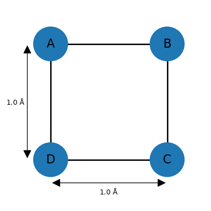
However, the upper bound of 100 is problematic since most distances between 0.5 and 100 Å are geometrically impossible given the other distances. Here, one can make use of the triangle inequality relationship, which states that for three points A, B, and C, distance AC can at most be AB + BC, meaning that the length of one side of a triangle must be less than or equal to the sum of the lengths of the other two sides. The inverse triangle inequality states that the minimum distance AC must be at least |AB − BC|.
While these relationships are valid for exact distances, very similar ones hold for upper and lower bounds. For example, applying the triangle inequality relationship to the three atoms A, B, and D of the square molecule indicates that the upper bound between D and B can be at most 2.0 Å, so the default value of 100 is lowered significantly. In general, the triangle inequality lowers some upper bounds, and the inverse triangle inequality raises some lower bounds.
RDKit Variants
The RDKit variants of the Distance Geometry (DG) approach are referred to as "experimental-torsion distance geometry" (ETDG), which includes experimental torsional-angle preferences, and "ETKDG," with additional "basic knowledge" (K) terms such as flat aromatic rings or linear triple bonds. ETKDG performs the following steps:
- Build a distance bounds matrix based on the topology, including 1–5 distances, but without van der Waals scaling.
- Triangle smooth this bounds matrix.
- If step 2 fails, repeat step 1, this time without 1–5 bounds but with vdW scaling, then repeat step 2.
- Pick a distance matrix at random using the bounds matrix.
- Compute initial coordinates from the distance matrix.
- Repeat steps 3 and 4 until the maximum number of iterations is reached or embedding is successful.
- Adjust the initial coordinates by minimizing a "distance violation" error function.
If the molecule consists of multiple fragments, they are embedded separately by default, which means that they are likely to occupy the same region of space.