Introduction
HQS Spin Mapper facilitates the derivation of effective spin-bath model Hamiltonians for real input materials from first principles.
Using the HQS Spin Mapper one is able to investigate a given input molecule or solid for the relevance of low energy spin physics and to determine the predominant spin degrees of freedom involved. The HQS Spin Mapper further allows for an automatic derivation of a model Hamiltonian describing the relevent spin degrees of freedom and their coupling to a fermionic environment.
Applications
An important use case of the HQS Spin Mapper is the study of materials with dominant spin physics (i.e. magnetism) on a quantum computer. For this purposes the package provides a method to d erive an accurate material-specific effective spin-bath model description from first principles, which can be used in a computation on a quantum device.
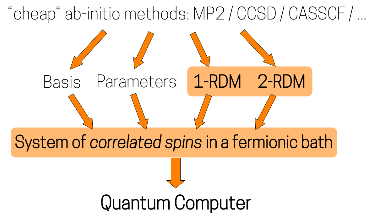
The figure above illustrates a procedure that allows for the simulation of real materials with relevant spin physics. The HQS Spin Mapper uses the results of preceeding electronic structure calculations to derive the spin-bath model description of the material that is suitable for simulation on near and intermediate term quantum computers.
-
In the first step, the basis orbitals of spin-like character are identified based on their local parity. This local parity is obtained using the one- and two-particle reduced density matrices (1-RDM and 2-RDM), which can computed using correlated ab-initio methods (e.g. MP2/CCSD/CASSCF/...).
-
In the second step, a mapping of the original Hamiltonian to a spin-bath model is performed by utilizing a generalized Schrieffer-Wolff transformation method.
For a detailed description of the full workflow please refer to the Theoretical background chapter.
Glossary
| CASSCF | Complete Active Space Self-Consistent Field |
| CCSD | Coupled Cluster with Single and Double excitations |
| MP2 | Møller-Plesset (Second Order) |
| 1-RDM | One Electron Reduced Density Matrix |
| 2-RDM | Two Electron Reduced Density Matrix |
Getting started
HQS Spin Mapper is a tool offered on HQStage to provide model analysis. It lets the user convert an electronic description of a system into a spin-based one. This gives the user more options for simulation methods and makes it possible to simulate these systems on quantum computers.
The HQS Spin Mapper module can be installed from HQStage
hqstage install hqs_spin_mapper
For detailed instructions on the installation see Installation.
A selection of applications of the HQS Spin Mapper for simple model systems and molecules are provided as Jupyter notebooks and are avalaible through HQStage
hqstage download-examples
Features
-
Automatic identification of spin degrees of freedom: The package offers two complementary local parity optimization routines. These identify linear combinations of basis orbitals with spin-like (or pseudo-spin-like) character. This information can be used to separate the system into effective spin and fermionic bath degrees of freedom.
-
Translation of Hamiltonian descriptions into fermionic operator representations: Tensor descriptions of the Hamiltonian, e.g. resulting from electronic structure calculations, can be translated into representations using fermionic algebraic operators. This allows for a quick and efficient computation of commutators.
-
Generalized Schrieffer-Wolff transformation method: The package offers a special Schrieffer-Wolff transformation routine that facilitates the transformation of generic fermionic Hamiltonians to effective spin-bath Hamiltonians. The accuracy of the transformed Hamiltonian is indicated by the local parity of the spin-like orbitals. Future extensions will allow for even more generic input systems and target effective Hamiltonians.
Installation
HQS Spin Mapper
Visit cloud.quantumsimulations.de/software, search for "HQS Spin Mapper" in the package list and select "Download". Follow the instructions on that page to install HQS Spin Mapper.
To use HQS Spin Mapper, you furthermore need to install the Intel Math Kernel Library (MKL), which is discussed in the next section.
MKL
If you desire, you can manually provide a version of the MKL by making sure
that the file libmkl_rt.so is found by the dynamic linker. That means,
that a system-wide installation should be found automatically.
If you use HQStage to install HQS Spin Mapper, you can install the MKL into an HQStage managed environment by running the following command.
hqstage envs install-mkl
Applications
Outline
- 1.1 Accepted input formats
- 1.2 Functionality: Spin-like orbital basis optimization
- 2.1 Preparation of input data for the Schrieffer-Wolff transformation
- 2.2 Functionality: Effective spin-bath model derivation
- 2.3 Extraction of tensor descriptions
- 2.4 Serialization with struqture
Functionality of the HQS Spin Mapper software package
HQS Spin Mapper software package contains a selection of modules which provide two major functionalities. The first functionality is the identification of orbital bases containing spin-like orbitals, i.e. orbitals with an occupancy of strictly a single electron. The second one derives effective spin-bath model Hamiltonians for the determined spin-like orbitals. The remaining modules handle input and output functionality.
1.1 Accepted input formats (hqs_spin_mapper.transformables)
HQS Spin Mapper currently accepts several different input formats for the Hamiltonian descriptions of a system (i.e. crystals and molecules). Some of the input formats store additional information about the system, which is, for example, needed for the determination of spin-like orbital bases or to reduce the computational of the spin-bath model derivation. There is also the possibility for the user to provide their own input format through the use of the supplied protocols.
Currently supported by default are:
LatticeBuilderconfiguration object instancesLatticeBuilderconfiguration data files as*.yml- Struqture FermionHamiltonianSystem object instances
- Data container (
Transformable_QuantumChemistry) including the one- and two-particle integrals specifying the Hamiltonian stored as numpy binary*.npyfiles. - Data container (
Transformable_Matrices) including the single particle picture matrices of the Hamiltonian as numpy array instances.
For each default input format, we provide a specific class derived from the Transformable class.
The Transformable object serves as the necessary input argument of the essential methods of the
hqs_spin_mapper package and are manipulated by these methods. The Transformable classes need to
satisfy the Supports_SW_Transformation protocol. Any object satisfying the
Supports_SW_Transformation protocol can be used with the functions provided by hqs_spin_mapper.
LatticeBuilder object instances and data files (Transformable_LatticeBuilder)
Given an instance of a LatticeBuilder object, it is easy to instantiate a
Transformable_LatticeBuilder object from, which can then be used as the input for the subsequent
functions. To instantiate the Transformable_LatticeBuilder object, use:
from hqs_spin_mapper.transformables import Transformable_LatticeBuilder

system = Transformable_LatticeBuilder(input_builder)
If the LatticeBuilder description of the system is stored in a valid *.yml file, the
Transformable_LatticeBuilder object is instantiated in the same way.
from hqs_spin_mapper.transformables import Transformable_LatticeBuilder

system = Transformable_LatticeBuilder(input_lattice_builder_yaml)
Struqture FermionHamiltonianSystem instances (Transformable_Struqture)
A Transformable_Struqture object can be directly instantiated from a
struqture_py.fermions.FermionHamiltonianSystem instance.
from hqs_spin_mapper.transformables import Transformable_Struqture

system = Transformable_Struqture(input_struqture)
Hamiltonians as numpy array instances (Transformable_Matrices)
The description of the Hamiltonian of a given system can be provided as a collection of matrices
and/or tensors respectively, in the single particle picture. The matrices and tensors first need to
be stored in a data container class called Hamiltonian_Matrices.
from hqs_spin_mapper.spin_mapper_protocols import Hamiltonian_Matrices

hamiltonian_matrices = Hamiltonian_Matrices(H0_uu=H0_uu,
                                            H0_dd=H0_dd,
                                            H0_ud=H0_ud,
                                            HU=HU,
                                            Jz=None,
                                            Jp=None,
                                            Jc=None)
The spin indices of the quadratic fermionic terms H0_uu,
H0_dd, H0_ud indicate the spin component of the electrons. If provided as a matrix, HU denotes
density-density interaction terms. If HU is provided as a tensor, more complex four index
interaction terms can be specified. The matrix Jz specifies interactions, Jp
specifies interactions, and Jc specifies interactions.
The quadratic Hamiltonian matrices H0_uu, H0_dd, H0_ud have to follow the convention
The matrices H0_uu, H0_dd, H0_ud have to be provided for three different combinations of the
spin directions , i.e. , and
.
If provided as a matrix (2-tensor), HU has to conform to
and if provided as a 4-tensor to
Using the Hamiltonian_Matrices instance, one can instantiate a Transformable_Matrices object
that satisfies the Supports_SW_Transformation protocol via
from hqs_spin_mapper.transformables import Transformable_Matrices

system = Transformable_Matrices(hamiltonian_matrices)
Electron integrals from electronic structure codes (Transformable_QuantumChemistry)
If the output of a preceding electronic structure calculations contains the one-electron and
two-electron integrals specifying the Hamiltonian, e.g. stored as numpy binary *.npy files, one
can construct a Transformable from the corresponding tensors via instantiation of a
Transformable_Matrices object as shown in the previous section.
from hqs_spin_mapper.spin_mapper_protocols import Hamiltonian_Matrices
from hqs_spin_mapper.transformables import Transformable_Matrices

H0_uu = np.load('h0_uu.npy')
H0_dd = np.load('h0_dd.npy')
H0_ud = np.load('h0_ud.npy')
HU = np.load('hu.npy')

hamiltonian_matrices = Hamiltonian_Matrices(H0_uu=H0_uu,
                                            H0_dd=H0_dd,
                                            H0_ud=H0_ud,
                                            HU=HU,
                                            Jz=None,
                                            Jp=None,
                                            Jc=None)

system = Transformable_Matrices(hamiltonian_matrices)
If the results from the preceding electronic structure calculations furthermore include the
one-electron density matrix (1-RDM) and the two-electron density matrix (2-RDM), one can instead
instantiate a Transformable_QuantumChemistry object. The Transformable_QuantumChemistry object
satisfies the Supports_Spin_Optimization protocol. This means that the object can be used as the
input argument for the spin basis optimization functionality of hqs_spin_mapper.
from hqs_spin_mapper.transformables import Transformable_QuantumChemistry
from hqs_spin_mapper.spin_mapper_protocols import Hamiltonian_Matrices

hamiltonian_matrices = Hamiltonian_Matrices(H0_uu=H0_uu,
                                            H0_dd=H0_dd,
                                            H0_ud=H0_ud,
                                            HU=HU,
                                            Jz=None,
                                            Jp=None,
                                            Jc=None)

rdm1_uu = np.load('rdm1_uu.npy')
rdm1_dd = np.load('rdm1_dd.npy')
rdm1_ud = np.load('rdm1_ud.npy')
rdm2 = np.load('rdm2.npy')

system = Transformable_QuantumChemistry(hamiltonian_matrices,
                                        rdm1=(rdm1_uu, rdm1_dd, rdm1_ud),
                                        rdm2=rdm2,
                                        tolerance=1e-1)
The input reduced density matrices have to adhere to specific conventions. The spin orbital optimization will otherwise yield non-physical results. We expect the following conventions for the reduced density matrices:
- single 1-RDM:
- spin-resolved 1-RDMs:
- single 2-RDM:
Input exclusively for spin-like orbital optimization (SpinFinder)
If the spin-bath model derivation functionality is not required, the user can instantiate a
SpinFinder object, which is the valid minimum input for the functions pertaining to the
determination of the spin-like orbital basis.
from hqs_spin_mapper.transformables import SpinFinder

rdm1_uu = np.load('rdm1_uu.npy')
rdm1_dd = np.load('rdm1_dd.npy')
rdm1_ud = np.load('rdm1_ud.npy')
rdm2 = np.load('rdm2.npy')

system = SpinFinder(rdm1=(rdm1_uu, rdm1_dd, rdm1_ud),
                    rdm2=rdm2)
Keyworded constructor arguments for Transformable objects
Attributes required by the Supports_SW_Transformation protocol:
system_size: Optional[int] = None: Number of orbitals in the system. This is automatically derived from the model description. (available forTransformable_Matrices,Transformable_QuantumChemistry)rotation_matrix: Optional[numpy.ndarray] = None: Basis transformation matrix between different orbital bases. The index denotes the orbital in the old basis and the orbital in the new basis. Default is the identity. (available forTransformable_LatticeBuilder,Transformable_Matrices,Transformable_QuantumChemistry)prefactor_cutoff: float = 1e-6: Terms of the Hamiltonian with coupling constant of absolute value smaller than the chosen value are discarded in the derivation of the spin-bath model (Schrieffer-Wolff transformation). (available forTransformable_LatticeBuilder,Transformable_Struqture,Transformable_Matrices,Transformable_QuantumChemistry)site_type: str = "spinful_fermions": Type of particles occupying the orbitals. (available forTransformable_Matrices,Transformable_QuantumChemistry)spin_indices: Optional[Set[int]] = None: User choice of orbitals to be treated as spin-like. The spin-like orbital optimization will add indices to this set. (available forTransformable_LatticeBuilder,Transformable_Struqture,Transformable_Matrices,Transformable_QuantumChemistry)
Attributes required by the Supports_Spin_Optimization protocol:
tolerance: float = 1e-1: Chosen discrepancy used in for a basis orbital to be considered spin-like, where denotes the local parity. (available forTransformable_QuantumChemistry,SpinFinder)optimization_steps: int = 4: Number of optimization loops to be performed. Parities are typically converged after 4 loops. (available forTransformable_QuantumChemistry, SpinFinder)
Other mutable attributes of Transformable objects
Attributes required by the Supports_SW_Transformation protocol:
generator: Union[ExpressionSpinful, ExpressionSpinful_complex]: Result for the generator of the Schrieffer-Wolff transformation.transformed_hamiltonian: Union[ExpressionSpinful, ExpressionSpinful_complex]: Result for the transformed fermionic Hamiltonian.
Atrributes required by the Supports_Spin_Optimization protocol:
immutable_indices: Set[int]: Indices of orbitals that are exempt from parity optimization.
Custom Transformable objects (hqs_spin_mapper.spin_mapper_protocols)
The user can create their own custom input format by implementing a class that satisfies the
protocols Supports_Spin_Optimization and/or Supports_SW_Transformation.
1.2 Functionality: Spin-like orbital basis optimization (hqs_spin_mapper.orbital_optimization)
HQS Spin Mapper provides the functionality to determine the optimal single-particle orbital
basis, in which a subset of the basis orbitals exhibits the maximum possible spin-like character.
We quantify the spin-like character of basis orbitals on the basis of their local parity
. For more details about the use of the local parity
as a measure for spin-like character, please consult the Theory section. An orbital
in the optimized basis is stored as spin-like if its local parity satisfies
, where corresponds to the value stored in the tolerance field of
the Transformable.
The spin_orbital_optimization function in the orbital_optimization module determines a basis
transformation which would optimize the local parities and stores the corresponding (proposed) basis
transformation in the rotation_matrix field of the Transformable object. The respective indices
of the spin-like orbitals in this optimized basis are stored in the spin_indices field of the
Transformable object. The spin_orbital_optimization function requires Transformable objects
that satisfy the Supports_Spin_Optimization protocol.
from hqs_spin_mapper.orbital_optimization import spin_orbital_optimization

spin_orbital_optimization(system)
Keyworded arguments
space_reduction: bool = True: If flag is set, the optimization is restricted to the indices not contained in theimmutable_indicesfield of theTransformable.fast_mode: bool = False: If flag is set, the rotations of the 2-RDM are performed approximately to reduce computation time.target: str = "minimum": Type of extremum to optimize for. Avalailable options are:minimum,maximum, andextremum._delta_sufficiently_spin_like: float = 1e-3: Exclude orbitals with initial parities and from the optimization search.
The function spin_orbital_optimization transforms the rdm1 and rdm2 to the optimized basis
(in order to save memory). The Hamiltonian tensors are not transformed. For the transformation
of the Hamiltonian tensors see the section on preconditioning of the input data.
The results of the optimized system are subsequently stored in the corresponding fields of the
Transformable object:
spin_indices = system.spin_indices
rotation_matrix = system.rotation_matrix

rdm1 = system.rdm1
rdm2 = system.rdm2
2.1 Preparation of input data for the Schrieffer-Wolff transformation (hqs_spin_mapper.preconditioning)
For the derivation of the spin-bath model, the spin_indices: Set[int] field of the Transformable
instance first requires a finite amount of indices. If the spin orbital optimization feature was
used, spin_indices of the Transformable have been set to feature the obtained spin orbitals
automatically. Otherwise spin_indices needs to be set manually by the user as e.g.:
spin_like_orbital_indices: Set[int] = {4, 9}

system.spin_indices = spin_like_orbital_indices
An intuitive choice for spin-like orbitals are orbitals with particularly strong repulsive local (i.e. on-site) interactions .
The preconditioning of the input data necessary for the subsequent Schrieffer-Wolff transformation
is done automatically by calling the preconditioning function on the Transformable object once.
Due to the side effects of the preconditioning function, we advise against multiple calls of the
preconditioning functions on the same Transformable object.
from hqs_spin_mapper.preconditioning import preconditioning

preconditioning(system)
The following tasks are performed by the preconditioning function:
- Generalization of the input interaction tensors
HU,Jz,Jp,Jcto a four index tensor description. - Rotation of the matrix and tensor descriptions to the optimized basis by rotation with the
rotation_matrix.
- If
apply_pre_diagonalization = True: Mean-field decoupling (ifSupports_Spin_Optimization) i.e. removal of bath exclusive interaction terms.
- If
apply_pre_diagonalization = True: Diagonalization of the quadratic bath Hamiltonian and transformation of the Hamiltonian tensors to the diagonal basis. - If
apply_cross_geometry = True: Re-indexing to place the spin indices in the middle of the system at , with defined as
x0 = (system.system_size // 2) - (len(system.spin_indices) // 2)
Keyworded arguments
apply_pre_diagonalization: bool = False: Perform a simplification of bath exclusive interactions and a diagonalization of the resulting quadratic bath Hamiltonian.apply_cross_geometry: bool = False: Move the spin indices to the center of the system (can speed up subsequent DMRG calculations).
2.2 Functionality: Effective spin-bath model derivation (hqs_spin_mapper.schrieffer_wolff)
With the input data preconditioned, the effective spin-bath model derivation becomes a simple call to
schrieffer_wolff on the Transformable object.
from hqs_spin_mapper.schrieffer_wolff import schrieffer_wolff

schrieffer_wolff(system)
The results of the derivation, namely the transformed Hamiltonian and the generator of
the transformation in
are stored in the Transformable object instances as:
transformed_hamiltonian = system.transformed_hamiltonian
generator = system.generator
Keyworded arguments
_max_length: int = 5: Size limit for the terms included in the generator._vector_space_cap: int = 1500000: Size limit of the vector space that the generator is determined from._max_krylov_space_dimension: int = 200: Size restriction of the Krylov space used in the SVD.rdm2: Optional[numpy.ndarray] = None: 2RDM for use in decoupling (currently not activated).
2.3 Extract tensor descriptions for the spin-bath model (hqs_spin_mapper.extract_couplings)
Using the functions contained in the extract_couplings module, one can retrieve the matrix and
tensor descriptions respectively of the spin-bath model Hamiltonian.
from hqs_spin_mapper.extract_couplings import extract_quadratic, extract_quartic

(H0_uu, H0_dd, H0_ud) = extract_quadratic(system)
HU = extract_quartic(system)
The matrices and tensor only contain the quadratic and quartic terms of the Hamiltonian respecitvely. The terms containing in excess of fermionic operators are not extracted.
2.4 Serialize the spin-bath model Hamiltonian with struqture (hqs_spin_mapper.struqture_interface)
The transformed Hamiltonian can be exported to an instance of
struqture_py.mixed_systems.MixedHamiltonianSystem for use in other HQS software or for
serialization.
from hqs_spin_mapper.struqture_interface import get_struqture_description

struqture_description = get_struqture_description(system)
Best practices
The HQS Spin Mapper software package contains a selection of modules which provide two major functionalities which are described in the "Applications" section in detail. On a high level, the first functionality is the identification of orbital bases containing spin-like basis orbitals, i.e. orbitals occupied by strictly a single electron. The second functionality facilitates the derivatioon of effective spin-bath model Hamiltonians for the detected spin-like orbitals. The remaining modules handle input and output functionality.
This section describes best practices in the application of HQS Spin Mapper.
Avoiding local extrema in the orbital optimization
Depending on the initial basis, it is possible that a single call to spin_orbital_optimization
fails to determine the true parity optimized basis. The pairwise optimization algorithm can get
stuck in local parity extrema of the parameter manifold. This behavior can be discouraged by using
the following procedure:
- Call the
spin_orbital_optimizationfunction on the input data withtarget="minimum". - Add the orbital indices that became spin-like to the
immutable_indicesof theTransformableinstance. - Call the
spin_orbital_optimizationfunction a second time on the updated input data with eithertarget="extremum"ortarget="maximum". - Call the
spin_orbital_optimizationfunction on the input data a final time withtarget="minimum".
Choosing a sensible value for prefactor_cutoff (Important to avoid memory overflow!)
To limit the system memory required for the Schrieffer-Wolff transformation algorithm, we recommend
adjusting the value of prefactor_cutoff. The terms of the input Hamiltonian in the optimized basis,
with an absolute coupling constant smaller than prefactor_cutoff will be excluded from the
Hamiltonian prior to the Schrieffer-Wolff transformation step. This is done because a large number
of small coupling constant terms slows down the SVD step of the transformation significantly, while
not significantly changing the result. In the evaluation of the commutators that yield the
transformed Hamiltonian, a larger number of terms can cause memory usage to exceed the system memory
and resulting in a fatal error. We recommend inspecting the size of the coupling constants of the
input Hamiltonian and choosing a value of prefactor_cutoff larger than the coupling constants that
can be considered insignificant. When in doubt, choose a larger value for prefactor_cutoff first
and then rerun the calculation with a slightly smaller value of prefactor_cutoff to check whether
the result is sensitive to the change in prefactor_cutoff. If the result remains sensitive,
we recommend gradually decreasing prefactor_cutoff and observing the memory usage.
We recommend to run the scripts or notebooks using the hqs_spin_mapper in an environment with a
set ulimit. The ulimit can be set in the terminal before running the Python interpreter via:
ulimit -v {maximum_desired_memory_in_kilobytes}
This way the process gets safely terminated without potentially crashing the system.
Estimation of the required memory
We provide a method for a rough estimate of the required memory resources to perform the
Schrieffer-Wolff transformation algorithm at the currently set value of prefactor_cutoff.
The function can be called on the Transformable object using:
from hqs_spin_mapper.preconditioning import (
    estimate_required_memory
)

estimate_required_memory(data)
The function estimate_required_memory prints an estimate of the necessary memory in GB. If the
estimated value exceeds the realistically available system memory, we recommended to increase the
value of the field prefactor_cutoff and to check the estimated memory requirement again.
Post-processing of the spin-bath model Hamiltonian
The result of the model Hamiltonian derivation is stored as an ExpressionSpinful object in the
transformed_hamiltonian field of the Transformable object. These objects offer a set of methods
that can be used for further manipulation of the transformed Hamiltonian. Here we list some useful
methods provided by the ExpressionSpinful class.
normalize(eps = 0.0): Sorts the operators in the terms of the Hamiltonian in a standardized fashion and removes terms with an absolute prefactor smaller than the valueeps.normal_order: Rewrites operators as creators and annihilators and normal orders them (creation operators to the left of annihilation operators).sort_descending: Sorts the terms in the expression by the absolute value of the coupling constants in descending order.sort_ascending: Sorts the terms in the expression by the absolute value of the coupling constants in ascending order.find(fermion): Returns the prefactor of the term containing the input operator.project_on_local_hilbert_subspace(x, condition): Projects the Hamiltonian on a subspace of the Hilbert space where theconditionis satisfied for sitex.conditionis the integer corresponding to a bit string, where the1-bit indicates thex-local state, the2-bit indicates , the4-bit indicates , and the8-bit indicates . The argumentcondition=6=4+2thus corresponds to , namely the singly occupied sitex.convert_to_spin_model(positions): Replace fermionic operators acting on thepositionswith spin operators assuming the identity .
A simple script to convert the transformed fermionic Hamiltonian to a true spin-bath Hamiltonian description is given by:
spin_bath_system = system.transformed_hamiltonian

for n in cast(List[int], system.spin_indices):
    spin_bath_system.project_on_local_hilbert_subspace(n, 6)

spin_bath_system = spin_bath_system.convert_to_spin_model(system.spin_indices)
Examples
Some example Jupyter notebooks of a spin-bath model derivation for the well-known Single Impurity Anderson Model (SIAM) and the Fermi-Hubbard Model are provided. The notebooks also include a spin optimization procedure for two molecules and the subsequent derivation of molecule specific spin models. The notebooks can be obtained by running the following command:
hqstage download-examples -m hqs-spin-mapper
The example notebooks contain the following examples
| Example | Filename |
|---|---|
| Real valued SIAM | siam_example.ipynb |
| Complex valued SIAM | complex_siam_example.ipynb |
| Real valued Fermi-Hubbard model | hubbard_example.ipynb |
| Kondo lattice chain model | kondo_lattice_example.ipynb |
| 1,3,5-Trimethylenebenzene | tmb_example/tmb_example.ipynb |
| Closed configuration Para-benzyne | pbz_spinfinder_example/pbz_spinfinder_example.ipynb |
There are furthermore a few simple example Python scripts avalaible in the examples directory of
the repository.
| Example | Filename |
|---|---|
| Real valued SIAM | siam_example.py |
| Complex valued SIAM | complex_siam_example.py |
| Real valued Fermi-Hubbard model | hubbard_example.py |
| Kondo lattice chain model | kondo_lattice_example.py |
Theoretical background
For users interested in the theoretical background behind the HQS Spin Mapper, we refer them to the sections Spin-like orbitals and Local Parity and Transformation of the many-body Hamiltonian. These sections are however not required reading for usage of the package.
In section Spin-like orbitals and Local Parity we
- define the notion of spin-like orbitals,
- propose the local parity as a metric for the spin-like character of orbitals,
- and present our parity optimiziation procedure as a way to determine the spin-like orbitals of a system.
The section Transformation of the many-body Hamiltonian describes
- the basic concept of the Schrieffer-Wolff transformation,
- our proposed extended Schrieffer-Wolff transformation method,
- and Schrieffer-Wolff transformation as a system of linear equations for unique block-offdiagonal operators.
Here, in section Full workflow we describe how the methods are combined into our workflow for deriving effective spin-bath model Hamiltonians for materials with relevant low-energy spin physics.
Full workflow
In the following, we outline the steps of the workflow that we use to derive an effective spin-bath model Hamiltonian from a first principles description of a material.
Computation of the required system information
We start with an ab-initio electronic structure calculation of the material to determine its ground state. The electronic structure method needs to be a post-Hartree-Fock or related method - this excludes density functional theory - to capture the effect of correlations in the two-particle reduced density matrix . From the electronic structure calculation we obtain the basis orbitals in which the Hamiltonian of the system is formulated, and the one-electron and two-electron integrals which specify the Hamiltonian description. For the ground state of the calculation we compute the one-particle and two-particle reduced density matrices and .
Determination of spin-like basis orbitals
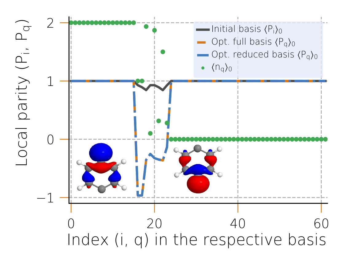
We utilize the reduced density matrices to assign a local parity to the basis orbitals i. We then perform pairwise rotations of the basis orbitals to determine the basis in which the local parities of the basis orbitals are extremized. If there exist optimized basis orbitals with , where we typically choose , we proceed with the subsequent steps of the workflow. If no spin-like orbitals are found, we terminate the workflow.
Schrieffer-Wolff transformation of the Hamiltonian
We use our Schrieffer-Wolff transformation approach to integrate out the valid terms of the Hamiltonian that modify the electron density in the spin-like orbitals, which leads to renormalized couplings of the electron spins in the spin-like orbitals to the environment. The valid terms are the ones that couple subspaces of the Hilbert space between which there exists a significant energy gap.
Construction of the effective spin-bath Hamiltonian
The transformed Hamiltonian is projected to the particular subspace of the Hilbert space where the electron density of spin-like orbitals is fixed to . Utilizing the identity fermionic operators acting on the spin-like operators are substituted with the corresponding spin operators. The resulting Hamiltonian is the effective spin-bath representation of the material.
Representation on a device (optional)
The effective spin-bath model Hamiltonian is re-expressed in terms of the spin operators that are realized on the specific device.
Spin-like orbitals and local parity
In the section Definition we define the notion of spin-like orbitals and in Local parity we propose the local parity as a metric for the spin-like character of orbitals. In Local parity optimization of the orbital basis, we present our parity optimization procedure as a way to determine the spin-like orbitals of a system.
Definition
We consider an orbital as being spin-like only if the electron density contained in it is strictly equal to one. This requires that the average electron density in the orbital satisfies . It furthermore requires that the fluctuations around this average electron density satisfy . Negligible fluctuations around the average electron density imply that electron density of the orbital does not affect the low-energy dynamics of the system and vice versa. Just an average electron density places no restrictions on the orientation and dynamics of the electron spin in the orbital . When both requirements are simultaneously met by the states in the low-energy Hilbert space, the dynamics of the electron density in the orbital , often referred to as the charge degree of freedom, become superfluous to the description of the dynamics of the system. The electron density in the orbital consequently couples to the remainder of the system exclusively via its spin degree of freedom. It is then sufficient to represent the degrees of freedom of the electron density contained in the orbital as a pure spin degree of freedom and to employ the associated spin operator algebra. The local Hilbert space of a spin degree of freedom is half the size of the local Hilbert space of a fermionic orbital and is furthermore naturally represented on a qubit. We therefore aim to determine each spin-like basis orbital or linear combinations thereof meeting both stated requirements, so that they can be represented as spins.Local parity
We propose the ground state local parity as a measure for the spin-like character of an orbital . The operator representation of the local parity reads where denotes the electron density in with electron spin quantum number and the electron density with quantum number respectively. The local Hilbert space of the orbital is spanned by the states,and the action of the local parity parity operator on these states reads For states where the orbital contains a single electron, the local parity operator returns the eigenvalue . For the remaining two basis states, returns the eigenvalue . Any state in the local Hilbert space that contains contributions from non singly occupied basis states hence satisfies with , because the resulting fluctuations in the electron density manifest themselves in strictly positive contributions to the local parity. An alternative and more useful operator representation of the local parity reads and its corresponding expectation value with respect to the many-body state can be expressed as where denotes the one-electron reduced density matrix (1-RDM) and denotes the two-electron reduced density matrix (2-RDM) respectively. If we choose , with a good approximation of the ground state of the system, we can identify orbitals for which , with , as spin-like orbitals of the system. In general, the spin-like orbitals of the system do not coincide with the basis orbitals. We therefore require a method to determine the set of orthonormal linear combinations of basis orbitals, for which the local parities most closely approach .
Local parity optimization of the orbital basis
We propose an iterative procedure to determine the particular orbital basis in which the local parities are extremal. For this we attempt a sequence of unitary pairwise rotations of the orbital fermionic operators given by with the same rotation being performed for the hermitian conjugates of the operators. From the reduced density matrices and , we can compute the local parity of an orbital , which results from the linear combination of orbitals and , as . The local parity is an analytic, -periodic function of the rotation angle . We find extremal points of the function in the domain from and select solutions that satisfy If a solution exists which satisfies and , we accept the rotation attempt and with rotation angle and we reject the rotation attempt otherwise. By repeating the procedure for each pair of basis orbitals and , we arrive at at an orthonormal basis in which the local parities have taken up extremal values. We then identify the orbitals of the resulting basis for which , with an arbitrary small, positive value, as the spin-like orbitals of the system. Basis orbitals with a local parity can be regarded as beneficial for the purpose of separating the system's spin degrees of freedom and their respective environment since they experience exclusively even number particle transfer, such that the spin degree of freedom of electrons occupying the orbitals becomes insignificant.Transformation of the many-body Hamiltonian
We discuss the basic concept of the Schrieffer-Wolff transformation in the section Perturbative similarity transformation. We detail our proposed extended Schrieffer-Wolff transformation method in sections Symmetry specification of block-offdiagonal operators and Schrieffer-Wolff transformation as a system of linear equations for unique block-offdiagonal operators.
Perturbative similarity transformation
In principle, any Hamiltonian can be completely diagonalized by means of a particular unitary transformation . In practice, finding the particular unitary transformation often requires a complete diagonalization of the Hamiltonian to begin with. Here we recap how a perturbative similarity transformation, namely the Schrieffer-Wolff transformation, can be used to determine an approximate transformation operator , or the generator thereof, which does not diagonalize the Hamiltonian fully, but yields a block-diagonal Hamiltonian instead. These blocks consist of the orthonormal states in the Hilbert space that share the a given choice of characteristics, e.g. the local particle quantum number . We will denote the set of terms in the Hamiltonian that are already block-diagonal in the initial basis as . The remaining terms connect different blocks, i.e are block-offdiagonal, and are denoted . The complete Hamiltonian thus reads
A unitary similarity transformation of the Hamiltonian is given by
where is an anti-hermitian operator. One refers to it as the generator of the Schrieffer-Wolff transformation. The key problem of the Schrieffer-Wolff transformation is finding the generator such that the transformed Hamiltonian becomes entirely block-diagonal. In order to arrive at an equation for one makes use of the Campbell-Baker-Hausdorff formula to expand
where for generators satisfying , with a suitable norm, one can approximate the expression as
Considering that commutators of pairs of block-diagonal operators or pairs of block-offdiagonal operators respectively generally become block-diagonal, while the commutators of block-diagonal operators with block-offdiagonal operators become block-offdiagonal, one chooses the equation
by which one can determine the generator which removes the block-offdiagonal terms of the Hamiltonian. If a solution exists, one can use
to simplify the expression for the transformed Hamiltonian
where the terms originating from contain the perturbative corrections arising from the consecutive application of two block-offdiagonal operators. A subsequent projection to the subspaces
yields the block-diagonal Hamiltonian
where denotes the distinct blocks of the Hilbert space.
Symmetry specification of block-offdiagonal operators
The block-offdiagonal part of the Hamiltonian consists of a sum of block-offdiagonal terms. These in turn comprise products of individually block-offdiagonal operators . In the following we detail a method to decompose generic block-offdiagonal operators into distinct components. Each of the components exclusively connects two distinct blocks of the Hilbert space , often associated with distinct quantum numbers of a symmetry of the system. A given block-offdiagonal operator satisfies
where denotes an arbitrary scalar and an arbitrary operator. Let be a diagonal operator in the initial basis. It can be identical to the symmetry operator differentiating the blocks of the Hilbert space, but it is not required to be. One can use the spectrum of to expand the operator as
where the different couple the target subspace associated with the eigenvalue of to other subspaces of the Hilbert space. If the operator satisfies then both subspaces, initial and final, coupled via are specified by the eigenvalue . This is possible for the fermionic creation and annihilation operators and . The coefficients are solutions to the equation The symmetry-specified block-offdiagonal operators satisfy where the operator denotes the hermitian conjugate of the operator .