Introduction

Raqet is a software package developed by HQS Quantum Simulations for the purpose of simulating the dynamics of quantum systems subject to noise.

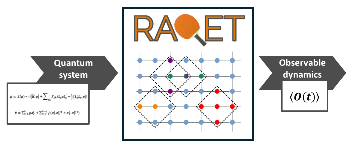
It performs these simulations in an efficient manner by taking advantage of the fact that in such noisy systems, decoherence limits the spread of quantum correlations. This can be used to reduce the level of complexity required to describe the physics of such a system, resulting in sub-exponential scaling of the equations of motion.

Applications

The factoring method is used to study local systems; that is, systems which are composed of individual sites, in which the total Hilbert space can be written as a tensor product of the Hilbert spaces of the individual sites. The primary requirement for using Raqet to simulate the dynamics of such a system is that a notion of distance can be defined between these sites, which is to be provided by the user. With such a notion of distance, Raqet determines how to reduce the complexity of the equations of motion which determine the evolution of the system.

Getting started

The HQS Raqet package can be installed via HQStage with the following command

hqstage install raqet-py

Examples of using Raqet to obtain the factorized dynamics of various physical systems can be found in the associated Jupyter Notebooks, which can be downloaded with

hqstage download-examples -m raqet-py

Features

The Python API documentation can be found here.

Theoretical Background

Here we briefly explain the theoretical ideas behind Raqet. While these ideas apply generally to any local quantum system, we focus here on the case of a system of interacting spin-1/2 particles (or qubits), since this is the type of system for which Raqet is currently implemented.

For the following discussion we consider the case of an \( N \)-qubit system, with Hilbert space \( \mathcal{H} \cong \mathbb{C}^{2^N} \) of dimension \( \mathcal{D} = 2^N \). The fundamental object of interest for any quantum system is the density matrix \( \rho \), with which we can compute the expectation value of any observable \( \mathcal{O} \) as

\[ \langle \mathcal{O} \rangle \equiv \mathrm{Tr}\left[\mathcal{O} \rho \right] \]

We denote by \( \{ A_n \} \) an orthonormal basis of the space of all traceless operators on the Hilbert space, normalized as

\[ \langle \langle A_n || A_m \rangle \rangle = \frac{1}{\mathcal{D}}\mathrm{Tr}\left[ A_n^{\dagger} A_m \right] = \delta_{nm}, \]

where the double bracket notation indicates an inner product on the space of operators. Any operator in our Hilbert space can be expressed as a linear combination of these operators and the identity,

\[ \mathcal{O} = \frac{1}{\mathcal{D}}\mathrm{Tr}\left[\mathcal{O} \right] I + \sum_{m=1}^{\mathcal{D}^2-1} a_{m} A_{m} \]

This includes the density matrix itself, which, taking into account the definition of the expectation value, can be written

\[ \rho = \frac{1}{\mathcal{D}} \left[ I + \sum_m \langle A_m \rangle A_m \right] \]

For a system of interacting qubits, it is customary to choose this basis to be the (Hermitian) elements of the Pauli group

\[ \{ A_n \} = \{ \sigma_1^{\alpha\left( n \right)} \sigma_2^{\beta\left( n \right)} \dotsb \sigma_N^{\omega\left( n \right)} \} \]

where \( \alpha, \beta, \ldots, \omega \in \{ I, x, y, z \} \). Performing the time evolution of the density matrix in an approximate manner is the main goal of Raqet.

Time Evolution of Quantum Systems

The goal of simulating the dynamics of a quantum system is to understand how certain observable quantities evolve with time. Since the density matrix of our system of qubits can be written as

\[ \rho = \frac{1}{\mathcal{D}} \left[ I + \sum_m \langle A_m \rangle A_m \right] \]

we see that tracking the time evolution of the density matrix is equivalent to tracking the time evolution of all of the expectation values \( \{ \langle A_n \rangle \} \). If the equation of motion for the density matrix is linear, then the expectation values will also satisfy some linear system of equations

\[ \frac{\mathrm{d}}{\mathrm{d} t} \langle A_n \rangle = \sum_m M_{nm} \langle A_m \rangle. \]

To determine this matrix \( M \) explicitly, we can insert the expression for the density matrix into Liouville's equation of motion for the density matrix,

\[ \frac{\mathrm{d}}{\mathrm{d}t}\rho = - i \left[ H, \rho \right], \]

where \( H \) is the Hamiltonian of the system, in order to find

\[ \sum_m \frac{\mathrm{d}}{\mathrm{d} t} \langle A_m \rangle A_m = -i \sum_m \langle A_m \rangle \left[ H, A_m \right]. \]

Taking the trace of both sides of this equation against \( A_n^{\dagger} \), we find

\[ \frac{\mathrm{d}}{\mathrm{d} t} \langle A_n \rangle = -\frac{i}{\mathcal{D}} \sum_m \mathrm{Tr}\left[ A_n^{\dagger} \left[ H, A_m \right] \right] \langle A_m \rangle, \]

which therefore identifies

\[ M_{nm} = -\frac{i}{\mathcal{D}} \mathrm{Tr}\left[ A_n^{\dagger} \left[ H, A_m \right] \right] \]

If our system is subject to noise in addition to Hamiltonian dynamics, one must simply make the replacement

\[ -i \left[ H, A_m \right] \to \mathcal{L} \left ( A_m \right ), \]

where \( \mathcal{L} \) is the full Lindblad time evolution operator,

\[ \mathcal{L} = -i \left[ H, \cdot \right] + \sum_{i} \gamma_{i} \left [ L_{i} \cdot L_{i}^{\dagger} - \frac{1}{2} \left \{ L_{i}^{\dagger} L_{i}, \cdot \right \} \right ] \]

with jump operators \( \left \{ L_{i} \right \} \). Repeating the above steps with this replacement, we find

\[ M_{nm} = \frac{1}{\mathcal{D}} \mathrm{Tr}\left[ A_n^{\dagger} \mathcal{L} \left ( A_m \right ) \right] = \langle \langle A_n || \mathcal{L} || A_m \rangle \rangle \]

which identifies \( M \) as simply the matrix representation of the superoperator \( \mathcal{L} \) in the basis of traceless operators.

Reducing the Complexity of the Equations of Motion

We see that the dynamical evolution of a quantum system can be understood by studying the time evolution of the expectation values of a given basis of traceless operators. The number of operators in such a basis will typically grow exponentially with the size of the physical system, making an exact simulation of quantum systems impractical beyond even relatively small system sizes. It is therefore necessary to make some sort of approximation when simulating most quantum systems of practical interest.

Raqet implements such a simplification by

1. Identifying a collection of operator expectation values which should be "unimportant" in some appropriate sense, and can therefore be omitted from the simulation

2. Determining how to modify the equations of motion in the absence of these unimportant expectation values.

How Raqet accomplishes these two tasks is explained in the following two sections.

Deciding which operators to discard

In order to decide which operators are "unimportant," Raqet makes a fundamental assumption about the physics of the system, which is that there exists a fundamental "length scale" beyond which correlations do not meaningfully spread. This assumption is plausible in local systems affected by noise, since the local interactions should generally result in a finite propagation speed for correlations, while in the presence of noise there is a time scale beyond which the system will decay to equilibrium, which is a state which will typically possess limited correlations. These two facts combined produce such an effective length scale. We can exploit this fact to eliminate degrees of freedom which extend over a region larger than this length scale.

In order to apply such a methodology to arbitrary quantum systems, we need a precise way to define a notion of "distance" between different "sites" in our quantum system. For now, we begin with the example of a simple lattice system, in which there exists an "obvious" notion of distance, and later we return to the more general case. An example of such a lattice system could be the one shown in the figure below. Each blue circle represents a quantum spin, with the distance between any two given positions being the shortest path through the links of the lattice. On such a lattice, we define the notion of the "diameter" of a collection of sites, which is the largest distance between any two sites in that collection. In the figure below, the dashed lines indicate collections of sites with a diameter of two.

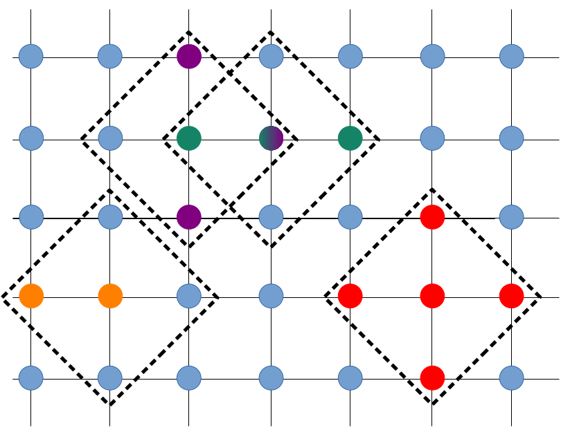
Any Pauli operator acting on such a system can be assigned a unique diameter. To see how, we consider the two sites colored in orange. The set containing only these two sites has a diameter of one, as this is (somewhat trivially) the largest distance between any two sites in this set. Any Pauli operator which involves these two sites can therefore be said to also have a diameter of one. For example, if these two sites were labeled as sites 1 and 2, then the operator \( \sigma_{1}^{z}\sigma_{2}^{z} \) would have a diameter of one. The other three collections of sites indicated in the figure, labeled with the colors red, purple, and green, all have diameters of two, and so any operators which involve those collections of sites would likewise have diameters equal to two.

With this definition, we can now state the fundamental approximation made by Raqet. To control the degree of approximation, a cut-off length scale is chosen. Any operator whose diameter is less than this cut-off scale is considered important, and is retained. All other operators are discarded.

Such an approximation is motivated by the notion of a Lieb-Robinson bound. In many local systems, there is a finite speed at which correlations can spread. If such a system is further subjected to noise, then this noise may ultimately drive the system into a steady state with limited correlations. The finite speed at which correlations spread, combined with the finite time over which noise will cause the system to undergo decoherence, leads to an effective distance scale over which correlations can never spread. Two sites which are further apart than such a distance scale can effectively never never develop correlations. If an operator contains two such sites, it would seem plausible that such an operator is "too big" to contribute important effects to the evolution of the system.

We emphasize here three important points about this condition.

First, we do not make any effort to "prove" why operators below a certain cut-off diameter should be important, nor do we attempt to derive what this cut-off should be. We simply take this assumption to be the defining approximation of Raqet. Whether or not this assumption is appropriate is ultimately determined by the performance of Raqet.

Second, we emphasize that the diameter is the key quantity when choosing which operators to keep, and not the number of sites involved in a Pauli operator. To clarify this point, we consider again the system indicated in the figure above, and imagine that we wish to control the degree of approximation by keeping all operators with a diameter of two or less. Any operator involving the sites in one of the colored sets (as well as many others) would be kept in this approximation. This includes, for example, any operators involving the sites colored in red, since even though there are five sites in this collection, the diameter of this set is still only two.

Third, our approximation does not correspond to making a partition of the system lattice. In the case that we choose to keep all operators with a diameter of two or less, we would keep (among others) operators which are defined on both the green and purple sets, even though these two sets overlap, and the combined region of overlap has a diameter of more than two.

More general notions of distance

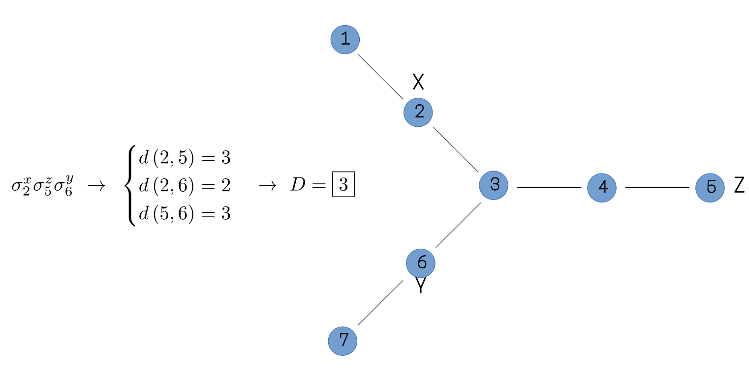
To apply these ideas to more general systems, we need to be able to generalize the concept of a distance function between two sites, beyond the case of simple lattice systems. In principle, this distance function can be any function which satisfies the mathematical definition of a metric. In practice, however, the distance function should ideally reflect something about the physics of the system. To see one example of how we might accomplish this, we consider the example system in the figure below. Such a system might represent a toy model of a molecule to be studied in an NMR experiment, with the sites corresponding to the nuclear spins of its constituent Hydrogen atoms. For such a system, we may wish to compute the diameter of, for example, the operator \( \sigma_{2}^{x}\sigma_{5}^{z}\sigma_{6}^{y} \). If we again consider the distance between any two sites to be the number of lattice links which must be traversed in order to travel from one site to the other, then we would assign a diameter of three to this operator, as shown in the figure.

In many physical systems, however, the couplings between individual sites in a system are not uniform. It would therefore seem natural to account for this lack of uniformity when determining the distance between different sites. One way to accomplish this is shown in the figure below, in which the connections between sites have been labeled with hypothetical Hamiltonian couplings. If we imagine the "length" of these individual connections to be inversely proportional to the corresponding Hamiltonian couplings, then the distance traveled between any two spins will now differ from the naive calculation, leading to a diameter of four for this operator, rather than three.

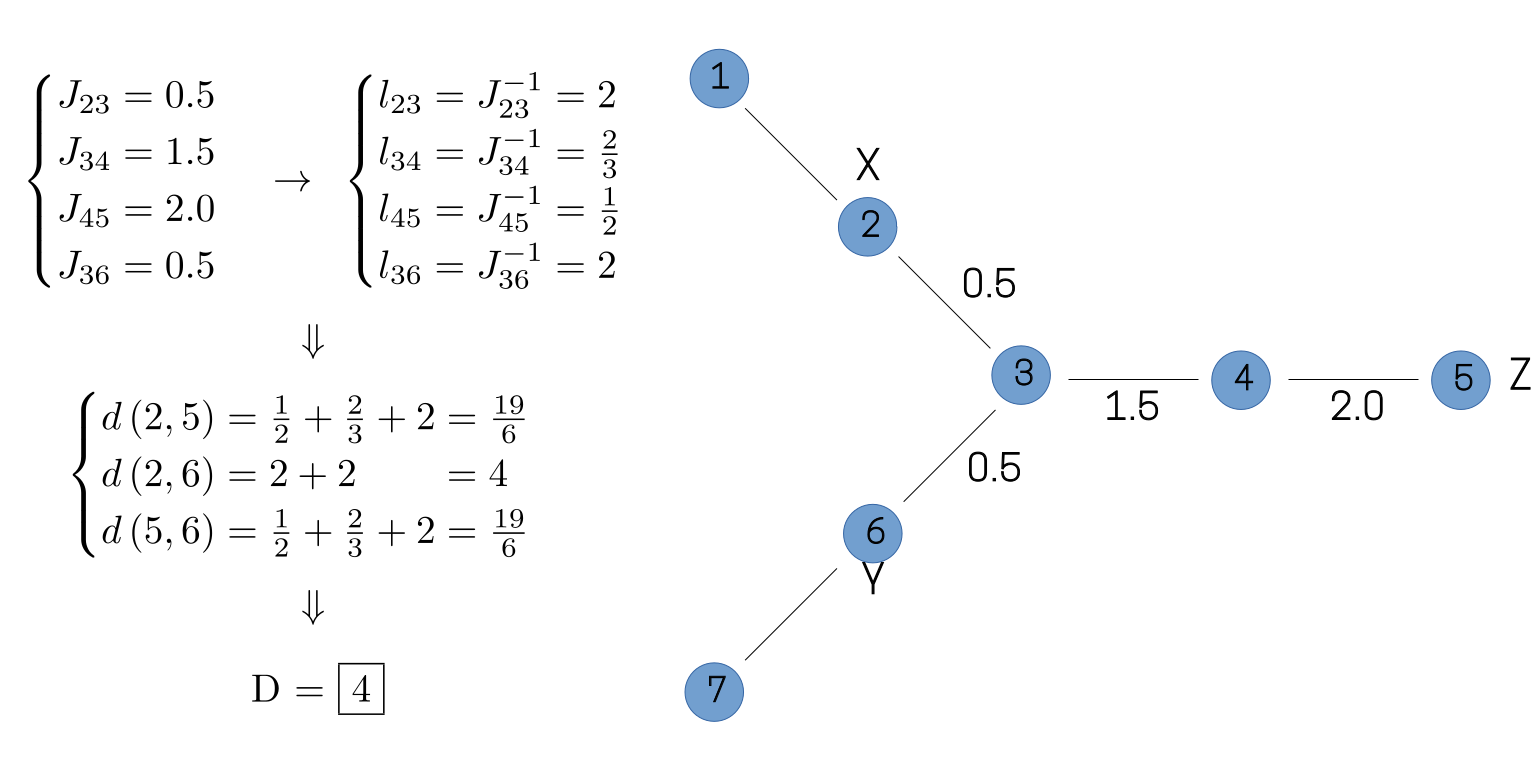
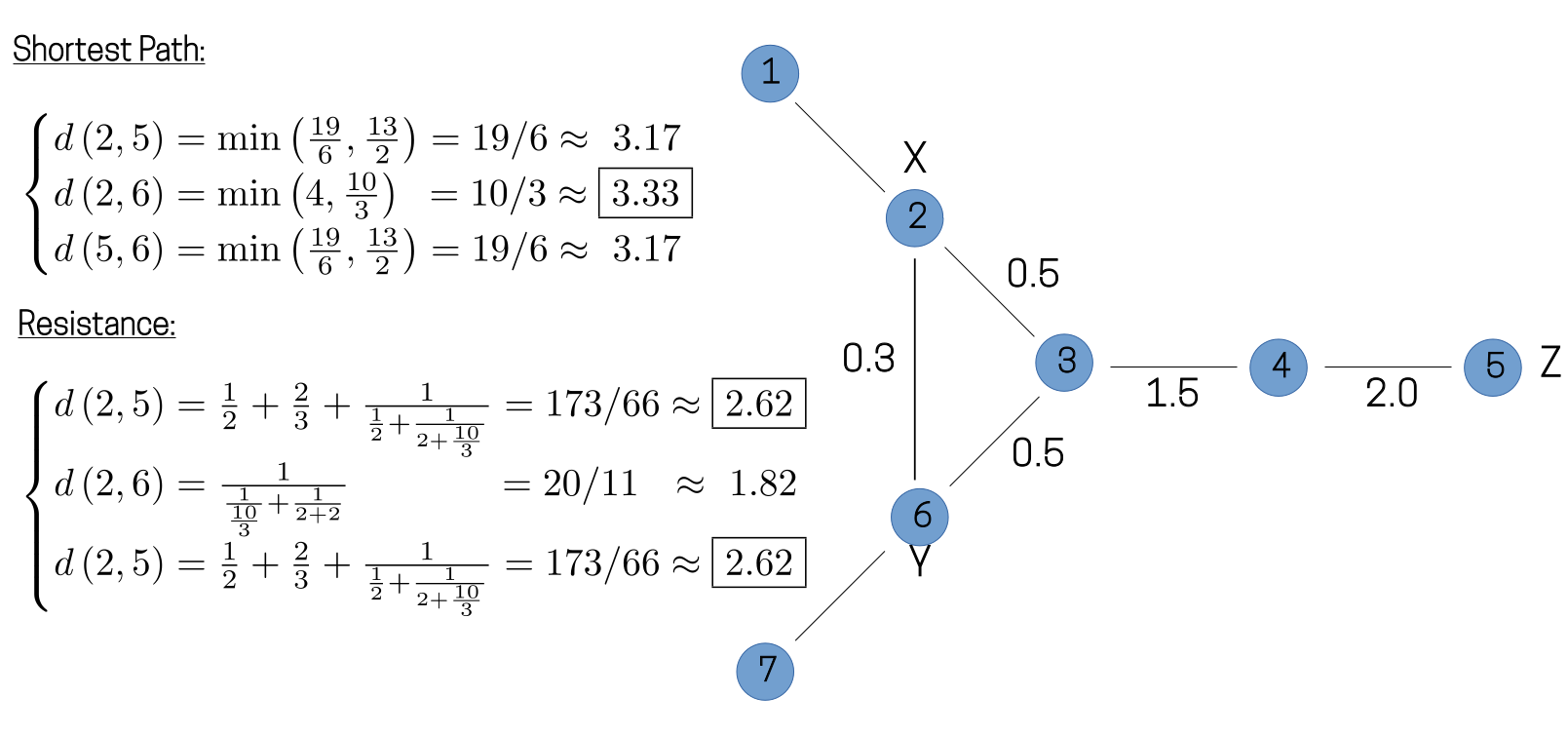
Of course, in most cases of physical interest, the Hamiltonian couplings will result in multiple possible paths between any two sites. In such a situation, there are several available options for defining a distance function. One option is to choose simply the shortest possible path between any two sites, while a somewhat more involved metric imagines the couplings to represent a sort of resistance network between sites, with the distance between any two sites now corresponding to the effective resistance between them. The choice of distance function will result in slightly different values for the diameter of our operator, as illustrated in the figure below.

While we could continue to refine our notion of distance for this example system, in practice, we have found reasonably good results by making use of the ideas we have developed so far. In some sense, the "best" possible distance metric for any given system should measure the amount of time it takes for correlations to develop between two sites, since the fact that correlations spread throughout the system at a finite speed is the underlying physical motivation for the method. Of course, knowledge of this type of information would generally require a solution to the dynamics, which is precisely what we wish to find using Raqet. Thus, some amount of physical intuition will always be necessary when postulating a notion of distance.

Modifying the Equations of Motion

Once we have made a decision regarding which operators to disregard during the evolution of our system, we still need to decide how to modify the equations of motion for the remaining operators. This is necessary because even if we have decided to neglect the time evolution of the "unimportant" operators, it is still possible for them to appear in the equations of motion. For example, one possible term in our original equations of motion might be

\[ \frac{\mathrm{d}}{\mathrm{d}t} \langle \sigma_1^x \sigma_2^y \rangle = \langle \sigma_1^x \sigma_2^y \sigma_3^z \rangle + \ldots \]

If we have made our approximation such that the operator \( \sigma_{1}^{x}\sigma_{2}^{y} \) is kept, but the operator \( \sigma_{1}^{x}\sigma_{2}^{y}\sigma_{3}^{z} \) is discarded, then we need to decide how to alter the right side of this equation in the absence of the discarded operator.

In general, there are many ways such a modification could be made, with some methods being more applicable than others depending on the particular problem at hand. Raqet currently supports two methods for modifying the equations of motion:

• Truncate : The simplest possible method of accounting for the omitted operators, in which we simply drop them from the equations of motion, effectively setting their expectation values to zero for the entire simulation.
• Ursell: A method which uses the concept of an "Ursell function" in order to express the omitted expectation value in terms of the expectation values which are kept. This is explained in more detail in the next section.

The Ursell Method

The idea behind the Ursell method is to replace the expectation value of an operator with a sum over all possible partitions of that expectation value. An example of such an approximation might look like

\[ \langle \sigma_{1}^{x}\sigma_{2}^{y}\sigma_{3}^{z} \rangle \to p \langle \sigma_{1}^{x}\sigma_{2}^{y} \rangle \langle \sigma_{3}^{z} \rangle + q \langle \sigma_{1}^{x} \rangle \langle \sigma_{2}^{y} \sigma_{3}^{z} \rangle + r \langle \sigma_{2}^{y} \rangle \langle \sigma_{1}^{x} \sigma_{3}^{z} \rangle + s \langle \sigma_{1}^{x} \rangle \langle \sigma_{2}^{y} \rangle \langle \sigma_{3}^{z} \rangle \]

for some coefficients p, q, r, and s. This "factoring" reflects the idea that the operator \( \sigma_{1}^{x}\sigma_{2}^{y}\sigma_{3}^{z} \) is "too big," and thus it can be approximated by "breaking it up" into smaller pieces.

To completely specify the method, we must determine these coefficients. The specific choice Raqet makes when determining these coefficients is based upon the notion of the joint cumulant, or Ursell function, of a collection of single-particle operators. If we have a collection of operators \( \{ \sigma_{i} \} \) on different sites, we define the joint cumulant of these operators to be

\[ \kappa \left ( \sigma_{1}, \dots, \sigma_{n} \right ) = \sum_{\pi} (-1)^{|\pi|-1} \left ( |\pi| - 1 \right )! \prod_{B \in \pi} \langle \prod_{i\in B}\sigma_{i} \rangle \]

In the above expression, the sum over \( \pi \) is a sum over all possible partitions of the collection of sites, \( |\pi| \) is the number of parts in the partition, and \( B \) represents a part inside of a partition. As a concrete example, we might have

\[ \kappa \left ( \sigma_{1}^{x}, \sigma_{2}^{y}, \sigma_{3}^{z} \right ) = \langle \sigma_{1}^{x} \sigma_{2}^{y} \sigma_{3}^{z} \rangle - \langle \sigma_{1}^{x} \rangle \langle \sigma_{2}^{y} \sigma_{3}^{z} \rangle - \langle \sigma_{1}^{x} \sigma_{2}^{y} \rangle \langle \sigma_{3}^{z} \rangle - \langle \sigma_{2}^{y} \rangle \langle \sigma_{1}^{x} \sigma_{3}^{z} \rangle + 2 \langle \sigma_{1}^{x} \rangle \langle \sigma_{2}^{y} \rangle \langle \sigma_{3}^{z} \rangle \]

We can use this definition to define our factoring formula. If we have an operator we wish to "factor" which involves single-particle operators on several sites, we find the appropriate factoring formula by setting the joint cumulant of these to zero,

\[ \kappa \left ( \sigma_{1}, \dots, \sigma_{n} \right ) = 0. \]

For our example above, this would correspond to

\[ \langle \sigma_{1}^{x} \sigma_{2}^{y} \sigma_{3}^{z} \rangle - \langle \sigma_{1}^{x} \rangle \langle \sigma_{2}^{y} \sigma_{3}^{z} \rangle - \langle \sigma_{1}^{x} \sigma_{2}^{y} \rangle \langle \sigma_{3}^{z} \rangle - \langle \sigma_{2}^{y} \rangle \langle \sigma_{1}^{x} \sigma_{3}^{z} \rangle + 2 \langle \sigma_{1}^{x} \rangle \langle \sigma_{2}^{y} \rangle \langle \sigma_{3}^{z} \rangle = 0 \]

This then implies

\[ \langle \sigma_{1}^{x} \sigma_{2}^{y} \sigma_{3}^{z} \rangle = \langle \sigma_{1}^{x} \rangle \langle \sigma_{2}^{y} \sigma_{3}^{z} \rangle + \langle \sigma_{1}^{x} \sigma_{2}^{y} \rangle \langle \sigma_{3}^{z} \rangle + \langle \sigma_{2}^{y} \rangle \langle \sigma_{1}^{x} \sigma_{3}^{z} \rangle - 2 \langle \sigma_{1}^{x} \rangle \langle \sigma_{2}^{y} \rangle \langle \sigma_{3}^{z} \rangle. \]

In some case, it may be necessary to apply this condition recursively. For example, if we had chosen our approximation such that the operator \( \sigma_{1}^{x} \sigma_{3}^{z} \) is also deemed "unimportant," then it should not appear in the equations of motion either. We can eliminate this operator by applying a similar factoring to it as well, so that

\[ \langle \sigma_{1}^{x} \sigma_{3}^{z} \rangle \to \langle \sigma_{1}^{x} \rangle \langle \sigma_{3}^{z} \rangle \]

Plugging this back into the first approximation and simplifying, we ultimately have

\[ \langle \sigma_{1}^{x} \sigma_{2}^{y} \sigma_{3}^{z} \rangle = \langle \sigma_{1}^{x} \rangle \langle \sigma_{2}^{y} \sigma_{3}^{z} \rangle + \langle \sigma_{1}^{x} \sigma_{2}^{y} \rangle \langle \sigma_{3}^{z} \rangle - \langle \sigma_{1}^{x} \rangle \langle \sigma_{2}^{y} \rangle \langle \sigma_{3}^{z} \rangle. \]

We emphasize here that setting a joint cumulant to zero is a way to find an approximate expression for an expectation value which we have discarded. It is not, however, a method for determining which operators to discard. In Raqet, the decision to discard an operator is always based on its diameter, and setting cumulants to zero is used to determine factoring expressions only after the list of important operators has been constructed. In this way, the factoring method differs from a standard cumulant expansion.

The Raqet User Interface

Raqet's user interface is based on the FactorMethod class, which can be imported and instantiated as follows

from raqet_py.factor import FactorMethod

my_method = FactorMethod()

Once we have a FactorMethod instance, we will be adding to it all the information necessary for running the simulation, and finally calling the compute_EOMs() method to obtain the equations of motion, appropriately factorized. The main information we need to add to the FactorMethod are

• The Hamiltonian (as a struqture_py.spins.SpinHamiltonianSystem) for the unitary time evolution;
• The Lindblad-type noise (as a struqture_py.spins.SpinLindbladNoiseSystem) for the non-unitary time evolution;
• The "connectivity" set used for deciding which operators are "too large"

More specifically, the connectivity set is the set of all pairs of sites whose distance is less than the cutoff length scale. This implies that it is the responsibility of the user to determine a distance function and a cutoff length scale, and then provide Raqet with a list of all pairs of sites whose distance is below this scale. It is important not to confuse this connectivity set with the list of all sites that are directly coupled (or "connected") through the Hamiltonian - two sites will appear in the connectivity set so long as their mutual distance is less than the chosen cutoff, regardless of whether they are directly coupled through the Hamiltonian.

Moreover, the operators whose time evolution we want to compute can be set with the method set_operator_heap. If these are not specified, Raqet will default to looking at the \( 3N \) single-site operators \( \langle \sigma^x \rangle \), \( \langle \sigma^y \rangle \), \( \langle \sigma^z \rangle \). Adding information to the FactorMethod instance is done as follows:

import numpy as np
from struqture_py.spins import SpinHamiltonianSystem, SpinLindbladNoiseSystem

number_spins = 5

# Define the Hamiltonian
hamiltonian = spins.SpinHamiltonianSystem(number_spins)
hamiltonian.set("0X1X", 1.0)
hamiltonian.set("0X", 1.0)
hamiltonian.set("1X3X", 1.0)
hamiltonian.set("2Y4X", 1.0)

# Define noise term
noise = SpinLindbladNoiseSystem(number_spins)

for q in range(number_spins):
    this_op = str(q) + "X"
    noise.add_operator_product((this_op, this_op), 1.0)

# Add connectivity information, as a set of pairs
connectivity = set()

# Assume distance and cutoff such that only 1D neighbors are "close"
for i in range(number_spins-1):
    connectivity.add((i, i+ 1))

# Set the Hamiltonian:
my_method.set_hamiltonian(hamiltonian)

# Set the noise:
my_method.set_noise(noise)

# Set the connectivity information
my_method.set_connectivity(connectivity)

With our FactorMethod instance all set, we can compute the factorized equations of motion, and print both the linear and nonlinear (i.e. factorized) parts

my_method.compute_EOMs()

print(my_method.linear_EOM())
print(my_method.nonlinear_EOM())

The nonlinear part of the equations of motion is represented as a dictionary whose keys represent terms like \( \langle \sigma^x_1 \rangle \langle \sigma^z_2 \sigma^y_3 \rangle \) as lists of PauliProduct, and whose values are the corresponding complex coefficients.