Custom Operators
Many algorithms in HQS Quantum Solver can be used with your own operator implementations. All that is required is that your implementation fulfills the requirements of the protocols used by the algorithm of interest.
Protocols
Protocols are a Python language feature that allows describing the requirements an object has to fulfill for being used in a particular part of the program. Whenever you encounter a protocol class in the type hints of a function or method, the protocol class defines which methods and properties the corresponding argument object is expected to have and the corresponding return type it has to provide, respectively. It is not necessary that your class inherits from the protocol class.
For example, the
evolve_krylov function
expects a operator argument which adheres to the
SimpleOperatorProtocol.
To be allowed to pass an object as operator, the object just needs
to implement all the methods and properties listed in
SimpleOperatorProtocol,
which are the shape and dtype attributes and the dot method.
Example
In this example we want to simulate the time evolution of a single spin in a magnetic field for different field stengths, i.e, we consider the Hamiltonian for different values of and measure the expectation value of . Instead of building a new operator for every value of we are interested in, we create a Hamiltonian class, that applies the correct value of on the fly. Avoiding recreation of operators can sometimes reduce the time of the computation. For a single-spin system, however, we will not see any benefit, because the system is too small. Nevertheless, we stick with this simple example for demonstration purposes.
We start by performing the necessary imports.
# Title    : HQS Quantum Solver Larmor Precession
# Filename : larmor_precession.py
import numpy as np
from scipy.sparse.linalg import eigsh
import matplotlib.pyplot as plt
from hqs_quantum_solver.spins import VectorSpace, Operator, spin_x, spin_z
from hqs_quantum_solver.evolution import evolve_krylov, observers
Next, we construct the and operators, and we set the initial state to an eigenvalue of the operator.
v = VectorSpace(sites=1, total_spin_z="all")
Sx = Operator(spin_x(site=0), domain=v)
Sz = Operator(spin_z(site=0), domain=v)

eigvals, eigvecs = eigsh(Sx, k=1)
state = eigvecs[:, 0]
We can now define the Hamiltonian class as a custom operator.
In this class, we need to define the shape and dtype property and
the dot method. Note that the implementation of the dot method
is required to have a parameter called out that when not equal to
None needs to be filled with the result of the operator application.
class Hamiltonian:
    def __init__(self, B):
        self.B = B

    @property
    def shape(self):
        return Sz.shape

    @property
    def dtype(self):
        return Sz.dtype

    def dot(self, x, out=None):
        result = -self.B * Sz.dot(x)
        if out is not None:
            np.copyto(out, result)
        return result
We can now pass instances of the Hamiltonian class to the evolve_krylov function, like any other operator provided by HQS Quantum Solver.
times = np.linspace(0, 1, 100)

Bs = [1, 2, 5, 10]
observations = np.empty((len(Bs), times.size))
for n in range(len(Bs)):
    B = Bs[n]
    result = evolve_krylov(Hamiltonian(B=B), state, times, observer=observers.expectation([Sx]))
    observations[n, :] = np.array(result.observations)[:, 0]

plt.plot(
    times, observations[0, :],
    times, observations[1, :],
    times, observations[2, :],
    times, observations[3, :],
)
plt.legend([f"$B = {B}$" for B in Bs])
plt.xlabel(r"$t$")
plt.ylabel(r"$\langle S^x \rangle$")
plt.show()
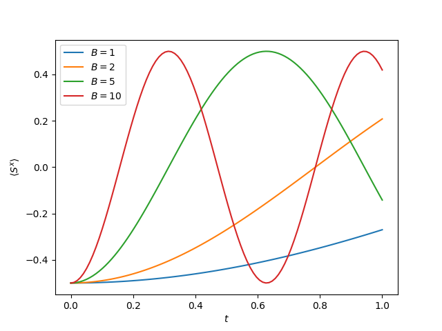
The expectation value of measuring .
Complete Code
# Title    : HQS Quantum Solver Larmor Precession
# Filename : larmor_precession.py
import numpy as np
from scipy.sparse.linalg import eigsh
import matplotlib.pyplot as plt
from hqs_quantum_solver.spins import VectorSpace, Operator, spin_x, spin_z
from hqs_quantum_solver.evolution import evolve_krylov, observers

v = VectorSpace(sites=1, total_spin_z="all")
Sx = Operator(spin_x(site=0), domain=v)
Sz = Operator(spin_z(site=0), domain=v)

eigvals, eigvecs = eigsh(Sx, k=1)
state = eigvecs[:, 0]

class Hamiltonian:
    def __init__(self, B):
        self.B = B

    @property
    def shape(self):
        return Sz.shape

    @property
    def dtype(self):
        return Sz.dtype

    def dot(self, x, out=None):
        result = -self.B * Sz.dot(x)
        if out is not None:
            np.copyto(out, result)
        return result

times = np.linspace(0, 1, 100)

Bs = [1, 2, 5, 10]
observations = np.empty((len(Bs), times.size))
for n in range(len(Bs)):
    B = Bs[n]
    result = evolve_krylov(Hamiltonian(B=B), state, times, observer=observers.expectation([Sx]))
    observations[n, :] = np.array(result.observations)[:, 0]

plt.plot(
    times, observations[0, :],
    times, observations[1, :],
    times, observations[2, :],
    times, observations[3, :],
)
plt.legend([f"$B = {B}$" for B in Bs])
plt.xlabel(r"$t$")
plt.ylabel(r"$\langle S^x \rangle$")
plt.show()