Combining Vector Spaces

The Jupyter notebook corresponding to this section can be found here.

In this guide you will learn how to run simulations with a large number of spins by computing on a subspace given by a restricted set of states. To demonstrate this approach, we consider the following spin system. We split the sites into $n_{1}$ sites that experience a strong interaction and $n_{2}$ sites that experience a weak interaction, while a magnetic field is acting on all sites. More precisely, we consider the Hamiltonian

$\hat{H} = - B j \sum \hat{S}_{j}^{z} + J_{strong} j = 0 \sum n_{1} - 2 \hat{S}_{j} \cdot \hat{S}_{j + 1} + J_{weak} j < k \sum R_{jk} \hat{S}_{j} \cdot \hat{S}_{k},$ where $B, J_{strong}, J_{weak} \in R$ and $R \in R^{n \times n}$ . Furthermore, we choose the entries in the strictly upper triangle of $R$ to be uniformly randomly distributed between $0$ and $1$ and the remaining entries to be zero.

The Hamiltonian is defined on the space $V = V_{1} \otimes V_{2}$ , where $V_{1}$ contains all possible spin states on the first $n_{1}$ sites and $V_{2}$ contains the states where at most one spin of the remaining sites is in the $↑$ state. While the number of states represented by $V_{1}$ grows exponentially with $n_{1}$ , the number of states represented by $V_{2}$ only grows linearly with $n_{2}$ . Thus, we can perform computations with large values for $n_{2}$ .

Imports and Parameters

Throughout this guide, we will make use of the following imports.

import numpy as np
from scipy.sparse.linalg import eigsh
import matplotlib.pyplot as plt

from hqs_quantum_solver.spins import (
    VectorSpace, Operator, magnetic_field_z, isotropic_interaction, spin_z)

Furthermore, we use the following parameters.

sites_part1 = 12  # Number of sites of the first part
sites_part2 = 50  # Number of sites of the second part

B = -1.5      # The magnetic field strength
J_strong = 1  # The strength of the strong interaction
J_weak = 0.2  # The strength of the weak interaction

Vector Spaces

We want to construct the Hamiltonian $\hat{H}$ of the system, which requires to define the vector space that the operator is defined on, first.

We start by defining the space $V_{1}$ , which we do by constructing a VectorSpace object from the spins module. The vector space object is defined by the states that it represents, which are in turn defined by the number of spins in the system (sites) and the restriction on the total spin polarization in $z$ -direction (total_spin_z). Since we do not want to restrict the total spin polarization, we just pass "all" for this argument.

v1 = VectorSpace(sites=sites_part1, total_spin_z="all")

To create the space $V_{2}$ , we need to combine two spaces. The first space just represents the state where all spins are in the $↓$ state, and the second space represents the states where just one spin is in the $↑$ state. The first one is characterized by a total spin polarization of $- \frac{n _{2} ℏ}{2}$ and the second one by a total spin polarization of $- \frac{( n _{2} - 2 ) ℏ}{2}$ . We want a vector space that represents the states represented by both spaces combined. Using the | (or the span method) the desired space is constructed from the individual spaces. Note that the total spin is specified in units of $\frac{ℏ}{2}$ .

v2 = (VectorSpace(sites=sites_part2, total_spin_z=-sites_part2)
      | VectorSpace(sites=sites_part2, total_spin_z=-sites_part2 + 2))

Finally, we can use the * operator to compute the desired tensor product $V = V_{1} \otimes V_{2}$ .

v = v1 * v2

The next step is to define the coefficient matrices.

Building Operators

Building an operator in Quantum Solver works by calling the constructor of the desired Operator class with an expression describing the operator and the vector space.

The expression describing the magnetic field can be obtained by using the magnetic_field_z function. By providing the coef argument, we can specify the magnetic field in $z$ -direction per site as a vector. This vector is constructed by the code below.

B_coef = np.full(v.sites, B)

To define the interaction part of the Hamiltonian, we want to use the isotropic_interaction function, which gives the desired expression when given an appropriate coefficient matrix. Looking at the documentation of the function shows that we can describe the term $J_{strong} j = 0 \sum n_{1} - 2 \hat{S}_{j} \hat{S}_{j + 1}$ by providing a matrix where the first $(n_{1} - 2)$ entries of the first upper off-diagonal are set to $J_{strong}$ and the remaining entries set to zero. This matrix is constructed as follows.

d1 = np.where(np.arange(v.sites - 1) < v1.sites - 1, 1, 0)
J_strong_mat = J_strong * np.diag(d1, 1)

The second term is represented by a coefficient matrix with random coefficients in $[0, J_{weak}]$ .

rng = np.random.default_rng(314159)

J_weak_mat = J_weak * np.triu(rng.uniform(0, 1, (v.sites, v.sites)), 1)

Now, that we have the coefficient matrices, we can build the Hamiltonian. The interaction term, however, maps onto states that are not part of the vector space $V$ . Oftentimes, this is an indicator for an error. Hence, we have to pass strict=False as an argument to the Operator constructor, to explicitly allow Quantum Solver to drop states not present in the vector space.

H = Operator(
    magnetic_field_z(coef=B_coef) + isotropic_interaction(J_strong_mat + J_weak_mat),
    domain=v,
    strict=False
)

Spectrum & Eigenvectors

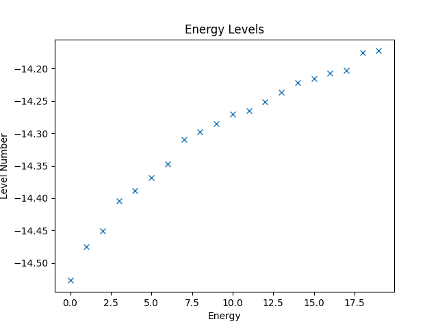
Having constructed the Hamiltonian, we can now use it to, e.g., compute the energy levels of the system. Since Quantum Solver operators are compatible with SciPy, we can directly use the eigsh function from SciPy to compute the eigenvalues.

eigvals, eigvecs = eigsh(H, k=20, which='SA')

The eigenvalues are the energy levels of the system and can be plotted as follows, while the resulting figure is shown below.

plt.figure()
plt.title('Energy Levels')
plt.xlabel('Energy')
plt.ylabel('Level Number')
plt.plot(eigvals, 'x')

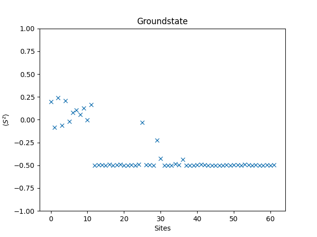
Another interesting quantity to look at is the expectation value of the spin polarization of the groundstate, i.e., $⟨ S_{j}^{z} ⟩ = ⟨ ψ ∣ S_{j}^{z} ∣ ψ ⟩$ for $j = 0, \dots, n_{1} + n_{2} - 1$ . The operator $S_{j}^{z}$ is provided by the spin_z function, and the application of the operator by the dot method, so the implementation is straight forward.

observables = [Operator(spin_z(site=j), domain=v) for j in range(v.sites)]

def spin_z_expectation(psi):
    return [np.vecdot(psi, o.dot(psi)) for o in observables]

The result can be plotted using the following code, and the resulting figure is shown below.

groundstate = eigvecs[:,0]

plt.figure()
plt.title('Groundstate')
plt.xlabel('Sites')
plt.ylabel(r'$\langle S^z \rangle$')
plt.ylim(-1, 1)
plt.plot(spin_z_expectation(groundstate), 'x')

plt.show()

The spin polarization of the groundstate.

Complete Code

# Title    : HQS Quantum Solver Combining Vector Spaces
# Filename : combining-spaces.py

# ===== Imports =====

import numpy as np
from scipy.sparse.linalg import eigsh
import matplotlib.pyplot as plt

from hqs_quantum_solver.spins import (
    VectorSpace, Operator, magnetic_field_z, isotropic_interaction, spin_z)

# ===== Parameters =====

sites_part1 = 12  # Number of sites of the first part
sites_part2 = 50  # Number of sites of the second part

B = -1.5      # The magnetic field strength
J_strong = 1  # The strength of the strong interaction
J_weak = 0.2  # The strength of the weak interaction

# ===== Vector Spaces =====

v1 = VectorSpace(sites=sites_part1, total_spin_z="all")

v2 = (VectorSpace(sites=sites_part2, total_spin_z=-sites_part2)
      | VectorSpace(sites=sites_part2, total_spin_z=-sites_part2 + 2))

v = v1 * v2

# ===== Building the Hamiltonian =====

B_coef = np.full(v.sites, B)

d1 = np.where(np.arange(v.sites - 1) < v1.sites - 1, 1, 0)
J_strong_mat = J_strong * np.diag(d1, 1)

rng = np.random.default_rng(314159)

J_weak_mat = J_weak * np.triu(rng.uniform(0, 1, (v.sites, v.sites)), 1)

H = Operator(
    magnetic_field_z(coef=B_coef) + isotropic_interaction(J_strong_mat + J_weak_mat),
    domain=v,
    strict=False
)

# ===== Plotting the Energy Levels =====

eigvals, eigvecs = eigsh(H, k=20, which='SA')

plt.figure()
plt.title('Energy Levels')
plt.xlabel('Energy')
plt.ylabel('Level Number')
plt.plot(eigvals, 'x')

# ===== Plotting the Spin Polarization =====

observables = [Operator(spin_z(site=j), domain=v) for j in range(v.sites)]

def spin_z_expectation(psi):
    return [np.vecdot(psi, o.dot(psi)) for o in observables]

groundstate = eigvecs[:,0]

plt.figure()
plt.title('Groundstate')
plt.xlabel('Sites')
plt.ylabel(r'$\langle S^z \rangle$')
plt.ylim(-1, 1)
plt.plot(spin_z_expectation(groundstate), 'x')

plt.show()