Introduction

To study the material properties of devices, it is necessary to include millions of sites in a materials science simulation. HQS Qolossal is a Python package that provides access to an efficient tight-binding solver with linear scaling in system size. This enables you to scale up the system size, allowing you to study, for example, semiconductor heterostructures or the effects of larger imperfections in a device. With HQS Qolossal you can directly analyze materials and devices or calculate effective parameters to improve the quality of finite element simulations.

The following quantities are supported:

• Density of states
• Trace of the resolvent
• Green's function
• Electrical conductivity
• Expectation value of user-defined operators
• Static linear response of user-defined operators to user-defined perturbations (e.g. susceptibilities)
• Spectral function
• Chemical potential
• Optical electrical conductivity
• Carrier density for semiconductors
• Electron mobility for semiconductors
• Electron diffusion coefficient for semiconductors
• Permittivity
• Normal incidence reflectivity
• Absorption coefficient

Theory

Linear scaling method

The linear scaling method we use is based on the expansion of the quantities of interest we want to study in terms of Chebyshev polynomials. These polynomials have been routinely employed in chemistry and physics and exhibit greater accuracy compared to other sets of orthogonal polynomials. In what follows, we give a brief introduction to the topic. For more details, see this reference.

The expansion of a function \(f: [-1, 1] \rightarrow {\rm R}\) in terms of Chebyshev polynomials of the first kind reads \[ \begin{aligned} f(x) & = \left[ \alpha_0 + 2 \sum\limits_{n=1}^{\infty} \alpha_n T_n(x)\right] \\ \alpha_n & = \int_{-1}^1 dx \frac{f(x) T_n(x)}{\pi \sqrt{1 - x^2}}, \end{aligned} \] where \(T_n(x)\) is the n-th Chebyshev polynomial of the first kind and \(\alpha_n\) is its corresponding moment. The Chebyshev polynomials benefit from the following advantageous recursion relation

\[ T_0(x) = 1, \quad T_1(x) = x, \quad T_{n+1}(x) = 2 x T_n(x) - T_{n-1}(x). \]

Although the above-mentioned expansion is correct and efficient, it can be problematic for the evaluation of the moments, due to the form of the denominator. A considerable simplification can be introduced by working with the modified orthogonal functions and the corresponding dot product:

\[ \begin{aligned} & \psi_n(x) = \frac{T_n(x)}{\pi \sqrt{1 - x^2}} \\ & \langle f\rvert\psi_n\rangle \equiv \int_{-1}^1 dx \sqrt{1 - x^2} f(x) \psi_n(x) = \int_{-1}^1 dx f(x) T_n(x). \end{aligned} \] Rewriting the expansion in this modified framework yields

\[ \begin{aligned} f(x) & = \frac{1}{\pi \sqrt{1 - x^2}} \left[ \mu_0 + 2 \sum\limits_{n=1}^{\infty} \mu_n T_n(x)\right]\\ \mu_n & = \int_{-1}^1 dx f(x) T_n(x), \end{aligned} \] which, as we will see later, allows for an efficient recursive calculation of the moments.

For what concerns our interest, the quantities we aim to represent in the basis of Chebyshev polynomials are functions of the Hamiltonian \(\hat{H}\) rather than a simple independent variable. Before expressing these functions as a Chebyshev expansion, it is important that the spectrum of the Hamiltonian lies within the interval \([-1, 1]\), since the Chebyshev expansion is only defined within this interval. If needed, the Hamiltonian should be rescaled by

\[ \tilde{H} = \frac{(H - E_C)}{E_W},\]

where \(E_C\) is the center of the original spectrum and \(E_W\) is its full width. For simplicity, in what follows, we omit the ~ sign on the Hamiltonian, however, we will always refer to the scaled Hamiltonian. The results obtained will need to be appropriately scaled back to fit the original spectrum, hence Hamiltonian ¹. The quantities of interest, which are functions of the (rescaled) Hamiltonian, can be expressed as a Chebyshev series by observing

\[ \begin{aligned} f(\hat{H}) & = \sum\limits_n f(\hat{H}) \lvert n\rangle \langle n\rvert = \sum\limits_n f(E_n) \lvert n\rangle \langle n\rvert = \sum\limits_n \sum\limits_m \mu_m T_m(E_n)\lvert n\rangle \langle n\rvert \\ & = \sum\limits_n \sum\limits_m \mu_m T_m(\hat{H})\lvert n\rangle \langle n\rvert = \sum\limits_m \mu_m T_m(\hat{H}) \end{aligned} \]

where the set \({\lvert n\rangle }\) is the set of single particle eigenfunctions of the Hamiltonian with eigenvalues \({E_n}\). As an example, let us explicitly write the expansion of the density of states, i.e.

\[ \rho(E) = {\rm Tr}\left[ \delta(E-\hat{H}) \right] = \sum\limits_n \langle n\rvert \delta(E-\hat{H}) \lvert n\rangle . \] The operator to be traced is, as we just pointed out, a function of the Hamiltonian. By inserting the resolution of the identity and using the manipulations shown above, we obtain

\[ \int dE' \delta(E' - \hat{H}) T_n(E') = \sum\limits_i \int dE' \delta(E' - \hat{H}) T_n(E') \lvert i\rangle \langle i\rvert = \sum\limits_i T_n(E_i) \lvert i\rangle \langle i\rvert = T_n(\hat{H}). \] The expansion of the density of states in terms of Chebyshev moments is then

\[ \begin{aligned} \rho(E) &= \sum\limits_n \mu_n T_n(E_n) \\ \mu_n &= \langle n\rvert T_n(\hat{H}) \lvert n\rangle . \end{aligned} \] This expression, though exact, is not particularly convenient, since it requires knowing all single-particle eigenfunctions \(\lvert n\rangle \). This would defeat the purpose of any other calculation, since the knowledge of these eigenstates and the corresponding eigenvalues defines any property of the system ². Nonetheless, the form presented above is used in our code to evaluate specific matrix elements of functions of the Hamiltonian, e.g. Green’s function matrix elements in the site basis, for which only a single evaluation is necessary. Fortunately, the calculation of the trace can be approximated in an efficient and accurate way through a stochastic evaluation ^{3 4}. In this approach, the trace of a general single particle operator \(\hat{A}\) is approximated as

\[ {\rm Tr}[ \hat{A} ] \simeq \sum\limits_{r=1}^R \langle r\rvert \hat{A} \lvert r\rangle ,\]

where the set of \({\lvert r\rangle }\) is a set of random states constructed from independent identically distributed random coefficients with zero mean. The vectors are normalized to 1, which ensures that the random vectors can indeed be considered states for all that concerns our calculations. This means, though, that when evaluating quantities such as the density of states, the average over the random states will be normalized to 1 instead of to the number of particles. Regarding accuracy, it has been shown ⁵ that the error of the approximation is proportional to \(1/\sqrt{N R}\), with N the size of the system and R the number of random vectors in the stochastic evaluation. This works in our favor as the accuracy increases with the system size, so much so that for a system with a billion sites, averaging over only a few \((<5)\) states is sufficient for most purposes ⁶: in this case \(1/\sqrt{N R} \lesssim 10^{-9}\).

Kubo formula for the conductivity

For the analysis of linear response, we use a method based on the Kubo formula. In this context, we will focus on the case of responses to electrical signals. According to the Kubo formula, the response of an operator \(\hat{A}\) to a zero-frequency (DC) perturbation is

\[ \langle \hat{A} \rangle = \Omega \lim\limits_{\tau, t \rightarrow \infty} \int^t_0 dt' e^{-t'/\tau }\int^\beta_0 d\beta' {\rm Tr}\left[ \hat{\rho}_{\rm eq} \hat{A}(0) \hat{\mathbf{J}}(-t' - i \hbar \beta') \right] \cdot \mathbf{E_0}, \]

where \(\Omega\) is the volume of the system, \( \tau \) is the intrinsic lifetime of the system, \( \hat{\rho}_{\rm eq} \) is the equilibrium density, \( \mathbf{E_0} \) is the DC perturbation and \( \hat{J} \) is the current operator. If the general operator \( \hat{A}=\hat{\mathbf{J}}_\alpha \), we have

\[ \label{eq_kubo_mb} \langle \hat{J}_\alpha \rangle = E_{0, \alpha}\left\{ \lim\limits_{\tau, t \rightarrow\infty} \int^t_0 dt' e^{-t'/\tau}\int^\beta_0 d\beta' {\rm Tr}\left[ \hat{\rho}_{\rm eq} \hat{J}_\alpha(t' + i \hbar \beta') \hat{\mathbf{J}}_\alpha(0) \right] \right\}, \]

where the volume has been ‘absorbed’ in the current, and we consider the spatially-averaged quantity. According to Ohm’s law, the quantity in the brackets in the equation above is the DC conductivity \(\sigma\). This formula simplifies considerably in the non-interacting case. Following the steps detailed in ⁷, we can rewrite the above equation as

\[ \langle \hat{A}(\mu) \rangle = \lim\limits_{\eta \rightarrow 0} - i \hbar \Omega \int dE' f(E' - \mu) {\rm Tr}\left[ \delta(E' - \hat{H}) \hat{A} \frac{1}{(\hat{H} - E') (\hat{H} -E' - i\eta)}(\hat{\mathbf{J}} \cdot \mathbf{E_0}) - h.c. \right], \] where the Fermi occupation function \(f(E)\) and the denominator of the fraction come from the density matrix. Additionally, the following propertiy has been used

\[ \begin{aligned} \int dE' F(E')\delta(E' - E_n) = F(E_n)\ \sum\limits_n F(E_n) \lvert n\rangle \lvert n \rangle \langle n\rvert = F(\hat{H}), \end{aligned} \]

where \(\lvert n\rangle \) are the single particle eigenfunction of the Hamiltonian with energy \(E_n\). Rewriting this equation in terms of Green’s functions, one obtains

\[ \langle \hat{A}(\mu) \rangle = i \hbar \Omega \int dE' f(E' - \mu) {\rm Tr}\left[ \delta(E' - \hat{H}) \hat{A} \frac{d G^+(E')}{dE'}(\hat{\mathbf{J}} \cdot \mathbf{E_0}) - h.c. \right], \]

where \(G^\pm(E')\) are the retarded and advanced Green’s functions. This formula is referred to as the Kubo-Bastin formula, and is equivalent to the Kubo formula for non-interacting systems.

If we focus on the conductivity, i.e. \(\hat{A} = \hat{J} = q \hat{V}/\Omega\), where q is the carrier charge and \(\hat{V}\) is the velocity operator, with some simple manipulations, we arrive to

\[ \sigma(\mu, T) = - \frac{2 \hbar e^2}{\Omega} \int dE' f(E' - \mu) {\rm Tr}\left[ \delta(E' - \hat{H}) \hat{V} \frac{d \operatorname{Im}\left[G^+(E')\right]}{dE'} \hat{V}\right], \] where we make use of \(G^+(E') - G^-(E') = -2i\operatorname{Im}\left[G^+(E')\right]\). Integrating by parts the last equation leads to

\[ \sigma(\mu, T) = - \frac{\hbar e^2}{\Omega} \int dE' \left[- \frac{\partial f(E' - \mu)} {\partial E'}\right] {\rm Tr}\left[ \delta(E' - \hat{H}) \hat{V} \operatorname{Im} \left[G^+(E')\right]\hat{V}\right], \] where the derivative of the Fermi function acts as a window selecting the energies around the chemical potential to contribute to the dissipative conductivity, as expected. The zero temperature limit of the above equation is the so-called Kubo-Greenwood formula

\[ \sigma(E) = \frac{\pi \hbar e^2}{\Omega} {\rm Tr}\left[ \delta(E' - \hat{H}) \hat{V} \delta(E - \hat{H}) \hat{V}\right], \] where we make use of the identity \(\operatorname{Im}\left[G^+(E)\right] = - \pi \delta(E - \hat{H})\). For simplicity the direction of the velocity operators has been omitted, but for calculating any element of the conductivity tensor one simply needs to use the velocity operators in the corresponding directions, i.e.

\[ \sigma_{xy} \propto {\rm Tr}[ \delta(E' - \hat{H}) \hat{V_x} \delta(E - \hat{H}) \hat{V_y}]. \] This formula can then be expanded in terms of Chebyshev polynomials by transforming the delta functions back into Green’s functions and evaluating the corresponding moments for the stochastic samples, as shown in ⁷, with the only difference being the normalization of the random states and, hence, the volume prefactor ⁸.

Velocity operator

As shown in the previous sections, to compute the conductivity of the system we need the velocity operator. In this section, we demonstrate how this is handled when the system is initialized via the Lattice Validator input. The velocity operator can be computed using Heisenberg’s equation of motion \(\hat{{V}} = i/\hbar [\hat{H}, \hat{R}]\), where \(\hat{R}\) is the position operator. While this is in principle a simple operation requiring two matrix-matrix multiplications and an addition, it becomes ill-defined for generic boundary conditions other than hard-wall. In fact, the position operator cannot be defined for periodic systems and the above-mentioned formula fails. This problem, though, can be circumvented by using the 'distance' information provided by the various bonds that make up the Hamiltonian. In fact, the translation vector associated with each bond will give us information about the real space displacement between the two unit cells connecting, i.e. all the spatial information we need to compute the commutator \([H, R]\). The periodic boundary conditions are then ‘automatically’ handled when implementing the recipe given by the translation associated with each bond to construct the full operator, much like the construction of the Hamiltonian. Note that it is not important where spatial origin is set, since this would simply introduce a contribution proportional to the identity to the position operator, which does not contribute to the value of the commutator. As an example, let us consider the case of an unevenly connected chain as shown in the following figure:

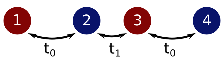
This system has the following Hamiltonian (on the lattice)

\[ H = \begin{pmatrix} 0 & t_0 & 0 & 0\\ t_0 & 0 & t_1 & 0\\ 0 & t_1 & 0 & t_0\\ 0 & 0 & t_0 & 0\\ \end{pmatrix}. \]

Considering a unit cell made of the two different sites, this Hamiltonian can equivalently be represented by the following bond information

\[ \begin{aligned} & (0, 0, 0)\, , \, \bar{t}_0 = \begin{pmatrix} 0 & t_0\\ 0 & 0 \end{pmatrix} \\ & (1, 0, 0) \, , \, \bar{t}_1 = \begin{pmatrix} 0 & 0\\ t_1 & 0 \end{pmatrix}, \end{aligned} \] where the vector represents the translation in terms of unit cells associated with the bond (hence \((0, 0, 0)\) is the bond within the unit cell), and \(\bar{t}_{0, 1}\) are matrices spanning the different sites of the unit cell and indicate the connections within the different sites (and their corresponding strengths). Since the Hamiltonian is the sum of the contributions of the two bonds, we can sum the velocity contributions associated with each bond. In this system only the x-component of the velocity operator will be non-zero. For the trivial translation associated with the bond \(t_0\), the commutator \([\bar{t}_0, {r}]\) can be directly evaluated, where \(\bar{t}_0\) is the first bond Hamiltonian from the previous equation and the matrix \(r\) is simply the position operator within the unit cell. For the second bond a similar approach can be used, but care has to be taken for the position operator. Let us now consider the subspace made of the original unit cell and the cell reached by the translation \((1, 0, 0)\), i.e. the displacement associated with the bond

\[ \bar{t}_1 = \begin{pmatrix} 0 & 0\\ t_1 & 0 \end{pmatrix}. \] The position operator in the x direction in the site basis in this subspace ⁹ reads:

\[ R_x = \begin{pmatrix} p^0_x & 0 & 0 & 0 \\ 0 & p^1_x & 0 & 0 \\ 0 & 0 & p^0_x + d_x & 0 \\ 0 & 0 & 0 & p^1_x + d_x \end{pmatrix} = \begin{pmatrix} \bar{r} & \bar{0} \\ \bar{0} & \bar{r}_d \end{pmatrix}, \] where \(\bar{0}\) is the \(2 \times 2\) null matrix, \(p^i_x\) is the position in the x direction of the site \(i\) and \(d_x\) is the displacement in the x direction corresponding to the lattice vector. The matrices \(\bar{r}\) and \(\bar{r}_d\) are the position operators in the original unit cell and the displaced one, respectively. Note that in general, the displacement vector is

\[ (l_1, l_2, l_3) \cdot (\mathbf{v}_1, \mathbf{v}_2, \mathbf{v}_3), \] where \(l_i\) is the translation associated with the bond for the i-th lattice vector \(\mathbf{v}_i\). Our example is the trivial case of a translation of magnitude one of a single lattice vector. In the same subspace, the Hamiltonian contribution of the (directional) bond is

\[ H^{t_1} = \begin{pmatrix} \bar{0} & \bar{t}_1 \\ \bar{0} & \bar{0} \end{pmatrix}. \] The position of non-zero block is determined by the directionality of the bond definition: if the translation were \((-1, 0, 0)\), i.e. hopping to the left, the non-zero block would be the lower left one. In terms of the block representation, it is trivial to evaluate the commutator

\[ V^{t_1}_x = \frac{i}{\hbar} [H^{t_1}, R_x] = \frac{i}{\hbar} \left[ \begin{pmatrix} \bar{0} & \bar{t}_1 \cdot \bar{r}_d \\ \bar{0} & \bar{0} \end{pmatrix} - \begin{pmatrix} \bar{0} & \bar{r} \cdot \bar{t}_1\\ \bar{0} & \bar{0} \end{pmatrix}\right], \] where the superscript \({t_1}\) denotes that the contribution to the corresponding quantities comes from the bond \(t_1\). Since the block structure of the resulting contribution to the velocity operator is the same as the bond, one can construct the velocity associated with each bond as \(v^{t_i}_x = i/ \hbar (\bar{t}_i \cdot \bar{r}_{d^i} - \bar{r} \cdot \bar{t}_i)\) and distribute these across the whole system in the same way as the Hamiltonian is constructed. The storage strategy will be the same as well, simply keeping track of the (intra-)inter-cell velocity contributions and the associated translations. In this sense the boundary conditions do not represent a problem from this perspective, because the correct behavior of the velocity operator is imposed by means of the distribution functions, i.e. how the sub-blocks are repeated in the matrix corresponding to the whole system.

Bibliography

Installation

For general information on installing the module and downloading the example notebooks, we refer you to the HQStage documentation.

Please note that HQS Qolossal is currently only supported on Linux.

Tutorial

In this section we will showcase the basic usage of HQS Qolossal. For more advanced examples, please visit the add example page reference.

To compute system properties with HQS Qolossal we simply need to initialize a Hamiltonian object. Once this has been correctly set up, you can invoke all available methods that directly compute the corresponding physical quantities -- no extra setup is required. HQS Qolossal offers several Hamiltonian implementations for ease of use. In the following tutorials we give more details on how to handle them.

Take a look at these pages for further details

• Initialization
• Calculations

Hamiltonian set up

HQS Qolossal supports different ways of defining Hamiltonians: via abstract definition, via directly providing the Hamiltonian in matrix form or as a linear operator. Additionally, you can add disorder to your systems.

Hamiltonian as a structured input

Setting up a Hamiltonian can be done via structured input using the Lattice Builder. Please check out its documentation for more information. In short, to define a lattice system, you need to specify which atoms/sites make up the unit cell, which bonds connect them, and other important information regarding the structure. The corresponding input dictionary can be directly handed to HQS Qolossal for initialization, for example:

from qolossal import HamiltonianSparse

unitcell = {
    'atoms': [
        {'id': 0, 'name': 'A', 'position': [0.0, 0.0, 0.0], 'e0': 0.0}
    ],
    'lattice_vectors': [[1.0, 0.0, 0.0]],
    'bonds': [
        {'id_from': 0, 'id_to': 0, 'translation': [1, 0, 0], 't': -1},
    ],
}

system = {
    'system_size': [1000, 1, 1],
    'site_type': 'spinless',
    'system_boundary_condition': ['PBC', 'HW', 'HW']
}

lb_input = {
    'unitcell': unitcell,
    'system': system
}

H = HamiltonianSparse(lb_input)

The script above initializes a 1D chain of length 1000 as a sparse Hamiltonian.

Hamiltonian as a matrix

Setting up a Hamiltonian with its matrix form is as simple as expected: we simply need to initialize the corresponding Hamiltonian class with it. Let's make the example of a 1D chain, whose non-zero entries in the Hamiltonian are just the two off-diagonals with value \(-t\)

import numpy as np
from scipy.sparse import diags
from qolossal import HamiltonianSparseDirect

# parameters
t = 1  # hopping amplitude
dimension = 10  # dimension of the chain
lattice_vector_length = 0.5  # in Angstroms

# initialize the hamiltonian matrix.
# NOTE: we use the csr format as this is what qolossal uses
diagonals = -t * np.ones(dimension)
Hamiltonian_matrix = diags(
    diagonals=[diagonals, diagonals],
    offsets=[1, -1],
    shape=(dimension, dimension),
    format='csr'
)

# initialize HamiltonianSparseDirect.
H = HamiltonianSparseDirect(
    H = Hamiltonian_matrix,
    total_volume = dimension * lattice_vector_length
)

This will initialize our Hamiltonian object and we will be able to start computing the systems properties. The above code will result in a RuntimeWarning: as we have not provided the velocity operators, the calculation of quantities that require these, such as the DC conductivity, will not work. To do so, we follow the same rationale

sites_position = np.arange(dimension) * lattice_vector_length
position_operator = diags(
    [sites_position],
    offsets=[0],
    shape=(dimension, dimension),
    format='csr'
)

# compute the velocity as V_x=i [H, r_x] (hbar=1)
velocity_x = 1.j * (
    Hamiltonian_matrix @ position_operator - position_operator @ Hamiltonian_matrix
)
# the velocity matrices for the y and z directions are just zeros.
velocity_y = velocity_z = diags(
    np.zeros(dimension),
    shape=(dimension, dimension),
    format='csr'
)

# initialize HamiltonianSparseDirect.
H = HamiltonianSparseDirect(
    H = Hamiltonian_matrix,
    total_volume = dimension * lattice_vector_length,
    velocity_times_hbar_matrices=[velocity_x, velocity_y, velocity_z]
)

Now we can proceed to compute velocity-dependent quantities as well.

Hamiltonian as a linear operator

To initialize the Hamiltonian with a linear operator we proceed exactly like for the matrix version.

import numpy as np
from scipy.sparse import diags
from qolossal import HamiltonianLinearOperator

# parameters
t = 1  # hopping amplitude
dimension = 10  # dimension of the chain
lattice_vector_length = 0.5  # in Angstroms

# initialize the hamiltonian matrix.
# NOTE: we use the csr format as this is what qolossal uses
diagonals = -t * np.ones(dimension)
Hamiltonian_matrix = diags(
    diagonals=[diagonals, diagonals],
    offsets=[1, -1],
    shape=(dimension, dimension),
    format='csr'
)


# we define the linear operator starting from the matrix for the example, but this can be
# done however one likes
def linear_operator(v: np.ndarray, out: np.ndarray) -> np.ndarray:
    """Apply Hamiltonian to vector.

    Args:
        v (np.ndarray): input.
        out (np.ndarray): preallocated output.

    Returns:
        np.ndarray: H @ v
    """
    # syntax used to make sure that the result is written in the already allocated space of "out"
    out[:] = Hamiltonian_matrix @ v
    return out


H = HamiltonianLinearOperator(
    linear_operator,
    dim=dimension,
    dtype=float,
    total_volume=dimension * lattice_vector_length
)

For the velocity we proceed in exactly the same way, ensuring the linear operators have the same signature as the Hamiltonian linear operator.

Disorder

HQS Qolossal can also add disorder to the system. Currently only local disorder is implemented: in this case a random potential is applied to the different sites. To add local disorder to a system we can simply specify its properties during the Hamiltonian initialization:

from qolossal import HamiltonianSparseDIrect

# ... initialization of all relevant arguments

H = HamiltonianSparseDirect(
    H = Hamiltonian_matrix,
    total_volume = dimension * lattice_vector_length,
    disDict={"type": "onsite", "distr": "uniform", "sigma": 0.1, "avg": 0}
)

where the disorder dictionary specifies the type of disorder (currently only "onsite"), the distribution type of the random potential (allowed: uniform, gaussian, laplace) and average value and standard deviation of the random potential.

Calculations

Once the Hamiltonian has been set up, we can call any method offered by HQS Qolossal to compute physical quantities of the defined system. Let's see the example of the density of states (DOS) for the 1D chain we have defined in the previous sections:

# ... initialize Hamiltonian

# scale the Hamiltonian to allow for the Chebyshev expansion to work
H.scaleH()

# calculate the density of states
dos, w = H.getDOS(
    NSamples=20,
    Order=200,
    NOmegas=2000
)

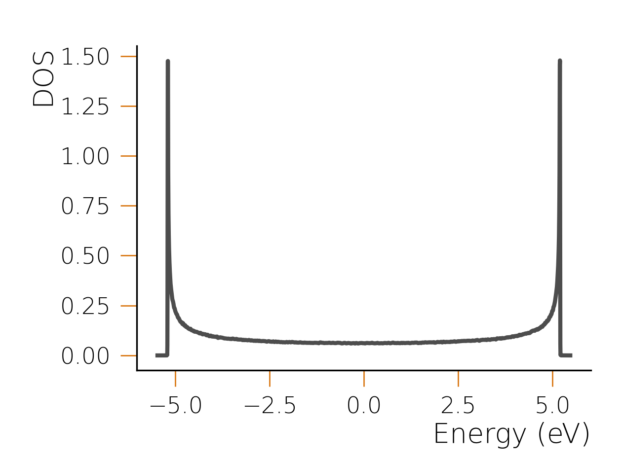
In this case, the arguments passed to the function control the number of random samples used for the DOS calculation, the order of the expansion and the number of frequencies at which to calculate the DOS. The above code will produce this following result:

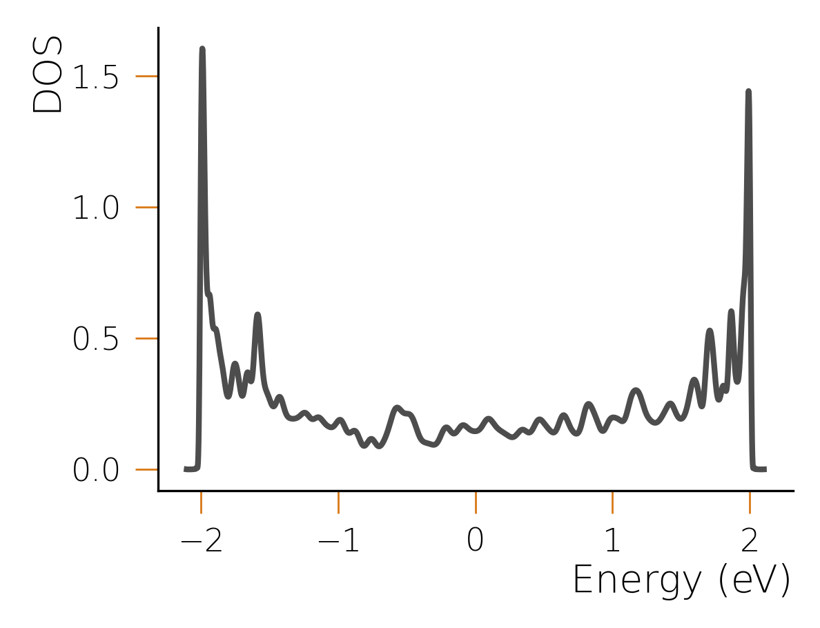
The wiggles in the result depend on the stochastic nature of the calculation and can be converged to the correct result by adjusting the convergence parameters. Larger systems (for which HQS Qolossal is made) require fewer random samples and, counterintuitively, converge faster to much smoother results thanks to self-averaging properties. In fact, using the same setup, but with a chain of size 20000, an order of the expansion of 1200 and 200 samples for the stochastic evaluation, we obtain the following result:

Units

This page serves as a reference for the input and output units in Qolossal. The symbol \( D \) in the following sections represents the dimensionality of the system.

Input parameters

Output Quantities