Background Information on Structure Conversion
This section provides further information on:
Background
The given list of references provides a summary of more technical aspects of the 3D structure conversion. More details can be found in the following sources:
- J. M. Blaney, J. S. Nixon, Distance Geometry in Molecular Modeling. Rev. Comput. Chem. 1994, 5, 299–335 (DOI:10.1002/9780470125823.ch6).
- S. Riniker, G. A. Landrum, Better Informed Distance Geometry: Using What We Know To Improve Conformation Generation. J. Chem. Inf. Model. 2015, 55, 2562–2574 (DOI:10.1021/acs.jcim.5b00654).
- S. Wang, J. Witek, G. A. Landrum, S. Riniker, Improving Conformer Generation for Small Rings and Macrocycles Based on Distance Geometry and Experimental Torsional-Angle Preferences. J. Chem. Inf. Model. 2020, 60, 2044–2058 (DOI:10.1021/acs.jcim.0c00025).
- RDKit documentation
Distance Geometry
The structure conversion routine of HQS Molecules makes use of the open-source cheminformatics
software RDKit, whose source code is available on GitHub.
Given the SMILES string or Molfile, an RDKit molecule object is created and
hydrogen atoms are added explicitly if needed.
Assuming a valid SMILES string is provided in the variable smiles,
the most basic steps are shown in the following code snipped:
from rdkit.Chem import AllChem

mol = AllChem.MolFromSmiles(smiles)
molH = AllChem.AddHs(mol)

status = AllChem.EmbedMolecule(molH)
As can be seen in the code above, in a first step a molecule object is created (MolFromSmiles function),
which contains 2D information about the molecule, such as the connectivity.
Since most hydrogen atoms are implicit in skeletal formulas and not included in the 2D structure,
but are indispensable for a 3D representation of the molecule, they need to be added in a second step (AddHs function).
However, the central function for generating 3D structures is the EmbedMolecule,
which returns 0 if the structure was generated successfully, and -1 otherwise.
This function computes a "3D embedding" based on variants of a stochastic approach referred to as
distance geometry (DG).
DG differs from standard Monte Carlo or molecular dynamics
techniques in that it directly generates structures to satisfy the geometric constraints of the model
instead of searching (almost) the entire conformational space to find appropriate structures.
As such, it can rapidly find one or more possible solutions but shares with other random methods
the inability to guarantee finding all of them.
Metric Matrix Method
The distance geometry (DG) approach described above is based on the assumption that purely geometric constraints can describe all possible conformations of a molecule, for which upper and lower distance bounds for all pairs of atoms are determined and represented in a distance bounds matrix. However, the key element of the DG technique is the metric matrix, , whose elements can be calculated from the vector product of the coordinates of atoms and , where is a matrix containing the Cartesian coordinates of the atoms. is a square symmetric matrix, and as such it can be decomposed as where the elements of the diagonal matrix are the eigenvalues and the columns of are the eigenvectors of . From the last two equations and the fact that has only diagonal entries it can be seen that This means that the Cartesian coordinates can be regenerated by multiplying the square root of the eigenvalues of with the eigenvectors . It has thus been shown that it is possible to convert three-dimensional atomic coordinates to the metric matrix and then regenerate them from it.
A crucial aspect in DG is that can also be derived directly from the distance matrix, , in which each component is the distance between atoms and . To this end, is first converted to , where each element is the distance between atom and the center of mass , where is the number of atoms. can then be calculated using the cosine rule, , and as seen before, the Cartesian coordinates can be obtained from .
Distance Bounds Matrix
Therefore, in order to get conformations of a molecule, it is necessary to provide a distance matrix, . Its components can be derived from the distance bounds matrix, which, as stated previously, contains upper and lower distance bounds for all pairs of atoms in a given molecule, determining the geometric constraints of the DG technique. But how can one define those bounds?
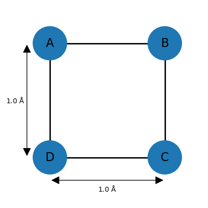
For example, imagine a square-shaped molecule with bond lengths of 1.0 Å. The upper and lower bounds for the neighboring atoms can thus be set to 1.0. Assuming that the atoms have van der Waals (vdW) radii of 0.25 Å, then all other lower bounds can be set to 0.5 (the default lower bound between any two atoms is the sum of of their vdW radii). However, the remaining upper bounds are not known, so a default of 100 is commonly chosen. This completes the entries of the distance bounds matrix, and a distance matrix can be generated from it by choosing distances randomly between the corresponding lower and upper bounds and entering them at appropriate places in .
However, the upper bound of 100 is problematic since most distances between 0.5 and 100 Å are geometrically impossible given the other distances. Here, one can make use of the triangle inequality relationship, which states that for three points A, B, and C, distance AC can at most be AB + BC, meaning that the length of one side of a triangle must be less than or equal to the sum of the lengths of the other two sides. The inverse triangle inequality states that the minimum distance AC must be at least |AB − BC|.
While these relationships are valid for exact distances, very similar ones hold for upper and lower bounds. For example, applying the triangle inequality relationship to the three atoms A, B, and D of the square molecule indicates that the upper bound between D and B can be at most 2.0 Å, so the default value of 100 is lowered significantly. In general, the triangle inequality lowers some upper bounds, and the inverse triangle inequality raises some lower bounds.
RDKit Variants
The RDKit variants of the Distance Geometry (DG) approach are referred to as "experimental-torsion distance geometry" (ETDG), which includes experimental torsional-angle preferences, and "ETKDG," with additional "basic knowledge" (K) terms such as flat aromatic rings or linear triple bonds. ETKDG performs the following steps:
- Build a distance bounds matrix based on the topology, including 1–5 distances, but without van der Waals scaling.
- Triangle smooth this bounds matrix.
- If step 2 fails, repeat step 1, this time without 1–5 bounds but with vdW scaling, then repeat step 2.
- Pick a distance matrix at random using the bounds matrix.
- Compute initial coordinates from the distance matrix.
- Repeat steps 3 and 4 until the maximum number of iterations is reached or embedding is successful.
- Adjust the initial coordinates by minimizing a "distance violation" error function.
If the molecule consists of multiple fragments, they are embedded separately by default, which means that they are likely to occupy the same region of space.