Introduction
The Bath Mapper is a module that can be used in conjunction with other Quantum Libraries by HQS Quantum Simulations GmbH. It supports the user in creating quantum mechanical objects which utilize the Bloch-Redfield master equation. This equation is a mathematical model, here used in quantum computing, to describe the dynamics of open quantum systems interacting with their environment (or "bath"). The Bath Mapper also provides functionality to allow further processing of the created objects.
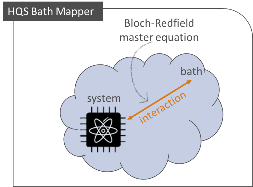
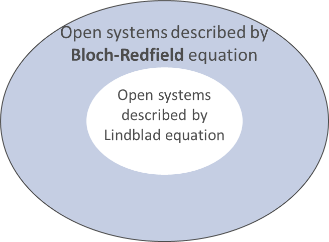
The Bloch-Redfield master equation is more general than the well-known Lindblad master equation. In particular, the Bloch-Redfield master equation does not make the assumption that the bath is Markovian, which allows the user to study open quantum systems as found in nature. The interactions of the system with the environment must be described by the spectral function, and the changes in the bath must be taken into account, making the computation more complex. What makes the HQS Bath Mapper so interesting, is that it explicitly uses the Bloch-Redfield master equation.
The user may find it hard to find a unified formulation of the Bloch-Redfield equation in textbooks, which is why we also provide the explicit form of it used in the HQS Bath Mapper here.
Applications
The main benefit of using the Bloch-Redfield equation instead of the Lindblad equation is that the user can study systems that are more likely to be found in nature. However, this approach is more specialized, which is why HQS provides the Bath Mapper module in addition to its struqture library. The Bath Mapper allows you to model more intricate interactions with the bath and more characteristics of the bath, by using the spectral function to represent the bath.
As mentioned above, another intrinsic advantage is that the user can study non-Markovian processes where the future quantum state depends on the past state and not only on the present state, which closely resembles real-world systems.

Here are some potential advantages and use cases of the Bath Mapper:
-
Modeling Open Quantum Systems: to study and understand real-world quantum systems, as they are rarely isolated and often interact with their environment.
-
Design and Optimization: since the Bath Mapper allows the user to manipulate the created objects, they can explore different settings and parameters.
-
Research and Development: using the Bath Mapper, researchers can model and manipulate quantum systems based on the Bloch-Redfield master equations to test hypotheses and explore new ideas.
-
Educational Purposes: as long as the access to the quantum computing hardware is a limited resource, such a tool can also be beneficial for educational purposes, helping students understand the underlying dynamics of open quantum systems.
The Bath Mapper can be used to create and manipulate objects based on the Bloch-Redfield master equation. The background physics associated with this is described in detail on the corresponding page.
Getting started
Install the package with the following command
hqstage install bath-mapper-py
The Bath Mapper is a module that can be used in conjunction with other HQS Quantum Libraries by HQS Quantum Simulations GmbH.
Please note that the HQS Quantum Libraries are currently only supported on Linux and MacOS.
Example implementations of the Bath Mapper functionality can be found here.
Features
The HQS Bath Mapper needs to be used in conjunction with the open-source HQS library struqture, designed for representing Hamiltonians and physical models. These objects are used as inputs and outputs for all of the functions below.
The functionalities associated with the SpinBRNoiseOperator and FermionBRNoiseOperators of the Bath Mapper are:
-
calculate_excitation_spectral_function: This function determines the bath excitation spectral function from a given Hamiltonian. Why it’s useful: The spectral function provides important information about how the environment (or “bath”) interacts with the user's quantum system. Understanding this interaction is crucial for predicting system behavior and designing experiments. -
spectral_function_to_coupling: This function converts a spectral function into a Hamiltonian that corresponds to the physical coupling between the system and the bath, describing how the spin system or fermion system interacts with its bosonic environment. Why it’s useful: By converting the spectral function into a Hamiltonian that represents the physical coupling, the user can better manipulate the interaction between their quantum system and its environment. This is important for tasks such as controlling decoherence and optimizing system performance. -
coupling_to_spectral_function: This function converts a Hamiltonian representing a physical coupling (describing how a spin system or fermion system is coupled to a bath) into a spectral function. Why it’s useful: This conversion helps the user to analyze and visualize the interaction in a different form, making it easier to interpret and apply in various contexts, such as theoretical studies or practical implementations.
For more detailed information on how to use these functions, including examples and specific inputs, please refer to the comprehensive documentation available here.
The API documentation is made available below.
Implementation and representation
When using the Bath Mapper, the user can create two primary types of objects: SpinBRNoiseOperator and FermionBRNoiseOperator. These objects are crucial for understanding and modeling noise in quantum systems.
-
SpinBRNoiseOperator: is used to model noise in systems that involve spin particles, such as electrons or atomic nuclei. In the context of quantum computing spins are used to encode quantum information and can be represented by Pauli operators. Spin noise can affect the coherence and stability of quantum states, so accurate modeling of this noise is important for applications in quantum computing. -
FermionBRNoiseOperator: is used to model noise in fermionic systems. In the context of quantum computing, fermions are represented by occupational operators. Fermionic noise is relevant in many areas of quantum mechanics and condensed matter physics, including the study of superconductors and quantum dots.
By creating and manipulating these objects the user can gain insight into how noise impacts their quantum system and develop strategies to mitigate its effects. For more detailed information on how to use these objects, including their specific methods and properties, please refer to the comprehensive documentation for spins and fermionic operators.
Further reading
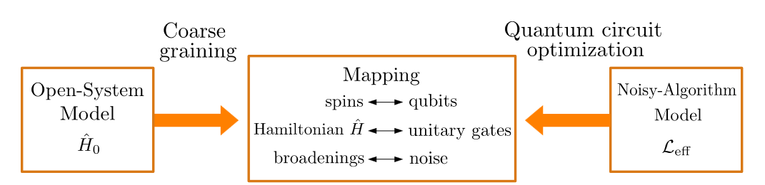
The underlying principles of the HQS Bath Mapper are detailed in our [scientific paper]((https://arxiv.org/pdf/2210.12138), which presents a quantum algorithm for simulating open system dynamics on quantum computers by leveraging noise. An overview of bath mapping, i.e., mapping between an open-system model and a noisy-algorithm model, is given in the figure below, with more details to be found in the scientific paper.
Background Physics
In this chapter we describe the details of the underlying quantum mechanics, with a focus on the two master equations relevant to the study of open quantum systems:
- Lindblad master equation,
- Bloch-Redfield master equation.
The Bloch-Redfield master equation is more general than the well-known Lindblad equation. In particular, the Bloch-Redfield master equation does not make the assumption of the bath being Markovian, which allows the user to study open quantum systems as found in nature. The interaction of the system with the environment must be described by the spectral equation, and the changes of the bath need to be taken into account, making the computation more complex.
Lindblad Master Equation
The Lindblad master equation, which can be derived from the von Neumann equation, is written as follows:
where
- is the density matrix of the qubits.
- The operators offer a basis for representation of the noise operators,
- while the matrix gives (generalized) noise rates.
Assumptions
This equation holds under the assumptions that
- the coupling between the system and the bath is weak,
- and that the bath is Markovian.
This corresponds to a flat bath spectral function. It is widely used in physics and chemistry to model open quantum system effects, and has the advantage of keeping the time-evolved density matrix physical (positive semi-definite).
Its main disadvantage is that it does not capture certain effects related to structured bath spectral functions, such as energy-change-dependent transition rates in thermalization when interacting with a finite temperature bath.
Bloch-Redfield Master Equation
The Bloch-Redfield master equation, which is the master equation utilized in this software module, relaxes the above assumptions of the Lindblad equation and thus generalizes the time-local master equation to cover also cases of structured spectral functions. This allows users to study important effects, such as energy-change-dependent transition rates, when studying open quantum systems with a finite temperature bath.
The Bloch-Redfield master equation can also be derived from the von Neumann master equation using second-order perturbation theory in the interaction with the bath. NOTE: While we will not re-derive the Bloch-Redfield master equation in this document, we will provide some information on how it relates to the code in this repository.
When derived, one obtains the following equation for the density matrix in the Schrödinger picture:
with , where
- is the bath correlation function in the time domain
- and are the system coupling operators
- the subscript refers to the interaction picture transformation.
A (positive time) Fourier transformation of the bath correlation function gives the energy-dependent transition rates and energy shifts by a relation of the form . Further derivation would be required to obtain the Bloch-Redfield superoperator from the above equations, which is beyond the scope of the bath-mapper user documentation.
Please note that the Bloch-Redfield equation simplifies to the Lindblad equation in the case of a flat spectral function, , where are now constants. This means that an open quantum system described by the Lindblad master equation can also be described by the Bloch-Redfield master equation, making the latter being more general in its applications. However, the Bloch-Redfield equation does not guarantee the physicality of the time-evolved density matrix in general. In particular, it should be used with caution when applied to spectral functions with sharp changes on the scale of the system-bath couplings.
Representing the Bloch-Redfield Equation (Spins)
SpinBRNoiseOperator: this Bath Mapper object is used to model noise in systems that involve spin particles, such as electrons or atomic nuclei. In the context of quantum computing spins are used to encode quantum information and can be represented by Pauli operators. Spin noise can affect the coherence and stability of quantum states, so accurately modeling this noise is important for applications in quantum computing.
Equation for Spins
As described in the background physics section, the Bloch-Redfield equation reads as follows:
with .
In the Bath Mapper library, we represent part of this equation. The SpinBRNoiseOperator represents
the spectral function, which is the Fourier transform of the correlation function in the time
domain, .
The SpinBRNoiseOperator
The Hamiltonian representing the couplings between the system and the bath for which the Bloch-Redfield formalism holds can be written as:
where are system operators and are bath operators. An example of a term would be , where the bath is assumed to be bosonic. (Note that the nature of the bath does not enter the Bloch-Redfield equation, only the spectral function matters.) It is important to note that terms cannot act on more than one spin in the Bath Mapper representation, i.e. terms such as are not allowed.
We can write the spectral function for a system of N spins with arbitrary coupling to a bath of bosonic modes respecting the above equation as follows:
where is the frequency of the bosonic modes, is the spectral function of the system operators and , and and are the bath operators. Examples for , , and are: , , and .
Using the SpinBRNoiseOperator
The SpinBRNoiseOperator is initialized with a list of frequencies for which to store the spectra.
Internally, the SpinBRNoiseOperator stores this list of frequencies, as well as a dictionary of
PauliProduct pairs with their corresponding spectral function. Each spectral function must have the
same number of points as the number of frequencies, and can have complex values.
Additionally, the SpinBRNoiseOperator has the following functions:
set- this takes a key(str, str)(representing the left and right PauliProducts) and a valueList[complex](representing the frequency-resolved spectral function corresponding to the key). It sets this combination of inputs in the internal dictionary.set_real- this takes a key(str, str)(representing the left and right PauliProducts) and a valueList[float](representing the frequency-resolved spectral function corresponding to the key). It sets the real part of a spectral function for two spin indices.set_imag- this takes a key(str, str)(representing the left and right PauliProducts) and a valueList[float](representing the frequency-resolved spectral function corresponding to the key). It sets the imaginary part of a spectral function.get- this takes a key(str, str)(representing the left and right PauliProducts) and returns the corresponding spectral function stored in the dictionary. If none is found, a list of zeros is returned.get_real- this takes a key(str, str)(representing the left and right PauliProducts) and returns the real part of the corresponding spectral function stored in the dictionary. If none is found, a list of zeros is returned.get_imag- this takes a key(str, str)(representing the left and right PauliProducts) and returns the imaginary part of the corresponding spectral function stored in the dictionary. If none is found, a list of zeros is returned.frequencies- returns the frequencies for which the spectral functions are defined.get_spectral_function_matrix- gets the matrix of the spectral function of a spin system at a specific energy index. It takes a spectral function indexint(the frequency index for which to return the matrix representation of the spectral function) and a number of spins (to build the correct size matrix) NOTE: The input for the couplings between the system spins and the bath (bosons) is of the form: , where . Therefore, the matrix we build is of size where is the number of system spins. The indexing of the columns is . The indexing of the rows is identical.resample- this function takes a list of frequenciesList[float]and resamples the current spectral functions according to this list of new frequencies.resample_interpolate- this function takes a list of frequenciesList[float]and resamples the current spectral functions via interpolation, according to this list of new frequencies.
Additionally, serialization functions such as to_json/from_json and to_bincode/from_bincode are available for
easy transfer of information.
Python Example
Below is a python snippet showing how to initialize and interface with the SpinBRNoiseOperator.
from hqs_quantum_libraries.bath_mapper import SpinBRNoiseOperator

frequencies = [0, 0.1, 0.2, 0.3, 0.4, 0.5, 0.6, 0.7, 0.8, 0.9]
br_operator = SpinBRNoiseOperator(frequencies)

z_z_spectral_function = [0.0, 0.0, 0.01, 0.012, 0.15, 0.28, 0.16, 0.08, 0.02, 0.01]
br_operator.set(("0Z", "0Z"), z_z_spectral_function)

assert br_operator.get_imag(("0Z", "0Z")) == [0.0 for _ in range(len(frequencies))]
assert br_operator.get(("0X", "0X")) == [0.0 for _ in range(len(frequencies))]
assert br_operator.frequencies() == frequencies

new_frequencies = [0, 0.025, 0.05, 0.075, 0.1, 0.125, 0.15, 0.175, 0.2, 0.225]
new_br_operator = br_operator.resample_interpolate(new_frequencies)

print(new_br_operator.frequencies())
print(new_br_operator.get(("0Z", "0Z")))
SpinLindbladNoiseOperator vs SpinBRNoiseOperator
As described in the Background Physics section, either the Bloch-Redfield master equation or the Lindblad master equation can be used to describe open quantum systems depending on the context and assumptions. struqture is the quantum computing library by HQS that utilizes the Lindblad equation.
The struqture object SpinLindbladNoiseOperator represents the noise part of the Lindblad master equation:
where is the density matrix of the qubits (spins). The operators offer a basis for the representation of the noise operators, while the matrix gives (generalized) noise rates.
Representing the Bloch-Redfield Equation (Fermions)
FermionBRNoiseOperator: this Bath Mapper object is designed to handle noise in systems involving fermions, which are particles like electrons that follow the Pauli exclusion principle, meaning that fermions don't commute. In the context of quantum computing fermions are represented by occupational operators. Fermionic noise is relevant in many areas of quantum mechanics and condensed matter physics, including the study of superconductors and quantum dots.
Equation for Fermions
As described in the spin operators section, the Bloch-Redfield equation for spins reads as follows:
with .
A similar construction can be used to represent fermions coupled to a (bosonic) bath. The operators would then be of the form , , or . As with the terms stored in the SpinBRNoiseOperator, the terms can only act on one fermion, i.e. terms such as are not supported.
Using the FermionBlochRedfieldNoiseOperator
The FermionBRNoiseOperator is initialized with a list of frequencies for which to store the
spectra. Internally, the FermionBRNoiseOperator stores this list of frequencies, as well as a
dictionary of FermionProduct pairs with their corresponding spectral function. Each spectral
function must have the same number of points as the number of frequencies and can have complex
values.
Additionally, the FermionBRNoiseOperator has the following functions:
set- this takes a key(str, str)(representing the left and right FermionProducts) and a valueList[complex](representing the frequency-resolved spectral function corresponding to the key). It sets this combination of inputs in the internal dictionary.set_real- this takes a key(str, str)(representing the left and right FermionProducts) and a valueList[float](representing the frequency-resolved spectral function corresponding to the key). It sets the real part of a spectral function for two spin indices.set_imag- this takes a key(str, str)(representing the left and right FermionProducts) and a valueList[float](representing the frequency-resolved spectral function corresponding to the key). It sets the imaginary part of a spectral function.get- this takes a key(str, str)(representing the left and right FermionProducts) and returns the corresponding spectral function stored in the dictionary. If none is found, a list of zeros is returned.get_real- this takes a key(str, str)(representing the left and right FermionProducts) and returns the real part of the corresponding spectral function stored in the dictionary. If none is found, a list of zeros is returned.get_imag- this takes a key(str, str)(representing the left and right FermionProducts) and returns the imaginary part of the corresponding spectral function stored in the dictionary. If none is found, a list of zeros is returned.frequencies- returns the frequencies for which the spectral functions are defined.get_spectral_function_matrix- gets the matrix of the spectral function of a spin system at a specific energy index. It takes a spectral function indexint(the frequency index for which to return the matrix representation of the spectral function) and a number of spins (to build the correct size matrix). NOTE: The currently accepted input for couplings between system fermions and bath bosons is of the form: . Therefore, the matrix we build is of size where N is the number of system fermions. The indexing of the columns is . The indexing of the rows is .resample- this function takes a list of frequenciesList[float]and resamples the current spectral functions according to this list of new frequencies.resample_interpolate- this function takes a list of frequenciesList[float]and resamples the current spectral functions via interpolation (according to this list of new frequencies).
Additionally, serialisation functions such as to_json/from_json and to_bincode/from_bincode are
available for easy transfer of information.
Python Example
Below is a python snippet showing how to initialize and interface with the FermionBRNoiseOperator.
from hqs_quantum_libraries.bath_mapper import FermionBRNoiseOperator

frequencies = [0, 0.1, 0.2, 0.3, 0.4, 0.5, 0.6, 0.7, 0.8, 0.9]
br_operator = FermionBRNoiseOperator(frequencies)

z_z_spectral_function = [0.0, 0.0, 0.01, 0.012, 0.15, 0.28, 0.16, 0.08, 0.02, 0.01]
br_operator.set(("c0a0", "c0a0"), z_z_spectral_function)

assert br_operator.get_imag(("c0a0", "c0a0")) == [0.0 for _ in range(len(frequencies))]
assert br_operator.get(("c1a1", "c1a1")) == [0.0 for _ in range(len(frequencies))]
assert br_operator.frequencies() == frequencies

new_frequencies = [0, 0.025, 0.05, 0.075, 0.1, 0.125, 0.15, 0.175, 0.2, 0.225]
new_br_operator = br_operator.resample_interpolate(new_frequencies)

print(new_br_operator.frequencies())
print(new_br_operator.get(("c0a0", "c0a0")))
FermionLindbladNoiseOperator vs FermionBRNoiseOperator
As described in the Background Physics section, either the Bloch-Redfield master equation or the Lindblad master equation can be used to describe open quantum systems depending on the context and assumptions. struqture is the quantum computing library by HQS that utilizes the Lindblad equation.
As in the spin case, the user should not confuse the objects FermionLindbladNoiseOperator and FermionBRNoiseOperator: the former is used to represent the Lindblad operators for fermionic systems in struqture, while the latter is used to represent the Bloch-Redfield spectral functions defined above.
Associated Methods
The HQS Bath Mapper must be used in conjunction with the open-source HQS quantum computing library struqture, which is designed to represent Hamiltonians and physical models. These objects are used as inputs or outputs of all the functions described below.
The functionalities associated with the SpinBRNoiseOperator and FermionBRNoiseOperator of the the Bath Mapper are described in this section.
calculate_excitation_spectral_function
This method determines the bath excitation spectral function for a given Hamiltonian. It takes the following inputs:
mode_fermion_system- A MixedHamiltonian composed of a spin/fermion system coupled to a non-interacting fermionic bath.temperature- The bath temperature. Enters later via the Fermi distributions of the bath.number_frequencies- The number of frequency points on which the excitation spectral function is calculated.
The function returns the SpinBRNoiseOperator/FermionBRNoiseOperator corresponding to the input
MixedHamiltonian.
In the case of a spin-fermion MixedHamiltonian
As described in the introduction section, the HQS Bath Mapper is tailored to functionalities that allow studies of the interaction between the system and the bath. Therefore, the function calculate_excitation_spectral_function is intended to deal only with couplings, and does not take into account any operators acting only on the system.
To use this function, the user defines a spin system coupled to a bath of free fermions. The system-bath coupling operator is of the form: , with summation over and where , but is not specified.
In the case of fermion-fermion MixedHamiltonian
The same applies to the fermion-fermion case, where the user defines a fermionic system coupled to a bath with of free fermions. Here, the system-bath operator is of the form: , with summation over and where is a system term and is a bath term. Also here, the operators acting only on the system are not taken into account, since the resulting spectral function describes only the interaction terms.
spectral_function_to_coupling
This method converts a spectral function into a Hamiltonian corresponding to a physical coupling, that describes how a spin system or a fermion system interacts with the bosonic bath to which it is coupled. It takes the following inputs:
spectral_function- A set of spectral functions fornumber_modesbaths.number_modes- The number of spins or fermionic modes in the system.
This function returns the calculated MixedLindbladOpenSystem.
In the case of a SpinBRNoiseOperator
If the input spectral function is a SpinBRNoiseOperator, the constructed MixedLindbladOpenSystem has one spin
subsystem (with number_modes spins) and 3 * number_modes bosonic subsystems, each with
frequencies.len() modes. This is because each spin is coupled to 3 bosonic baths, one for each of
the couplings. Additionally, each energy interval (and therefore each frequency)
contains one bosonic mode.
In the case of FermionBRNoiseOperator
If the input spectral function is a FermionBRNoiseOperator, the constructed MixedLindbladOpenSystem has one
fermionic subsystem (with number_modes fermionic modes) and number_modes * number_modes bosonic
subsystems, each with frequencies.len() modes. This is because each fermionic mode is coupled to
number_modes bosonic baths, as can couple to all terms. Additionally, each energy
interval (and therefore each frequency) contains one bosonic mode.
coupling_to_spectral_function
This method converts a Hamiltonian representing a physical coupling (describing how a spin system or fermion system is coupled to a bosonic bath) into a spectral function. It takes the following inputs:
mode_boson_system- A coupled open spin-boson system or fermion-boson system in the form of a MixedLindbladOpenSystem. The coupling between the fermion/spin and bosonic subsystems is limited to one single Pauli operator (in the case of a SpinBRNoiseOperator) or a operator (in the case of a FermionBRNoiseOperator) coupling to a single bosonic creation operator plus its Hermitian conjugate. The bosonic subsystem is limited to an interaction-free system, with the eigenfrequencies given directly by the coefficients of the occupation operators in the Hamiltonian . The Lindblad terms of the open system can only act on the bosonic subsystem and are limited to pure damping.frequencies- The frequencies for which every data point in the spectral function is defined.background- A constant background/offset that is included in the on-diagonal spectral function.additional_damping- An optional constant damping to be added to the one calculated from the open system.allow_empty_coupling- Allow a mixed system input with no coupling between subsystems. Will produce a zero spectral function.
This function returns the calculated spectral function.
In the case of a spin-fermion MixedHamiltonian
If the system part of the input MixedLindbladOpenSystem is a spin system, the
MixedLindbladOpenSystem should adhere to the following assumptions:
- The coherent system terms can be of any form, as they are not taken into account here.
- The coherent pure bosonic (bath) terms should be interaction-free, and should therefore only be of the form
- The coherent coupling terms between system and bath should be limited to one single Pauli operator coupling to a single bosonic creation operator plus its Hermitian conjugate:
- The noise terms should only act on the bosonic bath and should be limited to pure damping.
In the case of fermion-fermion MixedHamiltonian
If the system part of the input MixedLindbladOpenSystem is a fermionic system, the
MixedLindbladOpenSystem should adhere to the following assumptions:
- The coherent system terms can be of any form, as they are not taken into account here.
- The coherent pure bosonic (bath) terms should be interaction-free, and should therefore only of the form
- The coherent coupling terms between the system and the bath should be limited to operator coupling to a single bosonic creation operator plus its Hermitian conjugate:
- The noise terms should act only on the bosonic bath and should be limited to pure damping.
Chain Selection and Mapping
Candidate Creation
Given a device and a chain length, the bath-mapper library contains functions to create all possible (simple) chains of system qubits, where each system qubit is coupled to either one or two bath qubits.
create_candidates_bilinear: This function finds all of the simple chains with the given number of system qubits (chain length), where each system qubit is coupled to an associated bath qubit.chain_with_environment_candidates: This function finds all of the chains with the given number of system qubits (chain length), where each system qubit is coupled to an associated bath qubit. This function differs from the one above in that thecreate_candidates_bilinearonly accepts aSquareLatticeDeviceas input, while this function accepts any device implementing theChainWithEnvironmentDevicetrait.create_candidates_trilinear: This function finds all of the simple chains with the given number of system qubits (chain length), where each system qubit is coupled to two associated bath qubits.
Since there is no optimization here, in the worst case these functions should scale to produce candidates, where is the number of qubits in the device.
We call these candidate chains, as they can they can then be the input for the selection algorithms we have.
Candidate Selection
Given a device and a list of candidates, these functions select the best chain of system qubits with associated bath qubits in the candidate list.
Similar to the candidate creation, we have two functions for candidate selection:
select_optimised_bilinear_chain: accepts bilinear chains.select_optimised_trilinear_chain: accepts trilinear chains.
The user can select the optimization chosen for these chains, and we invite the user to look into this further in the Python API documentation.
Broadening of Bath Qubits
The broadenings function offers the functionality to calculate the broadening of a chain of bath qubits, where we define the broadening for each bath qubit as:
where
- is the damping rate of the qubit
- is the depolarization rate of the qubit
- is the dephasing rate of the qubit.
Examples
Examples of the implementation of the Bath Mapper's functionality can be found below.
from struqture_py import mixed_systems, spins, bosons  # type: ignore
from hqs_quantum_libraries.bath_mapper import (  # type: ignore
    coupling_to_spectral_function,
    SpinBRNoiseOperator,
    spectral_function_to_coupling,
)
import numpy as np

# Use three boson baths
bath_energies = [0, 1, 2]

# Use three boson baths
bath_broadenings = [0.1, 0.2, 0.3]

# Couplings to spin 0
couplings_0 = [0.3, 0.1, 0.3]
# Couplings to spin 1
couplings_1 = [0.2, 0.4, 0.2]

# Create a new mixed system with one spin and one boson subsystem
Hnew = mixed_systems.MixedLindbladOpenSystem(
    1,
    1,
    0,
)

# Set bath energies
for bath_index, be in enumerate(bath_energies):
    index = mixed_systems.HermitianMixedProduct(
        # Identity spin operator
        [spins.PauliProduct()],
        # Create a Boson occupation operator
        [bosons.BosonProduct([bath_index], [bath_index])],
        [],
    )
    Hnew.system_set(index, be)

# Set bath energies
for bath_index, bb in enumerate(bath_broadenings):
    # create the index for the Lindblad terms.
    # We have pure damping
    index = mixed_systems.MixedDecoherenceProduct(
        # Identity spin operator
        [spins.DecoherenceProduct()],
        # Create a Boson occupation operator
        [bosons.BosonProduct([], [bath_index])],
        [],
    )
    Hnew.noise_set((index, index), bb)


# Set couplings, use pure ZZ coupling
for bath_index, c in enumerate(couplings_0):
    index = mixed_systems.HermitianMixedProduct(
        # Identity spin operator
        [spins.PauliProduct().z(0)],
        # Create a Boson coupling  operator (always a + a^dagger)
        [bosons.BosonProduct([], [bath_index])],
        [],
    )
    Hnew.system_set(index, c)


# Set couplings, use pure ZZ coupling
for bath_index, c in enumerate(couplings_1):
    index = mixed_systems.HermitianMixedProduct(
        # Identity spin operator
        [spins.PauliProduct().z(1)],
        # Create a Boson coupling  operator (always a + a^dagger)
        [bosons.BosonProduct([], [bath_index])],
        [],
    )
    Hnew.system_set(index, c)

print("Newly created system")
print(Hnew.__repr__())

# Create a spectral function from Spin-Bath-System
frequencies = np.linspace(-0.5, 4, 100)
spectral_function = coupling_to_spectral_function(Hnew, frequencies)

print("Spectrum frequencies")
print(spectral_function.frequencies())

print("Spectrum for 0, 0 spin indices with Z-Z coupling")
print(spectral_function.get(("0Z", "0Z")))

print("Spectrum for 0, 1 spin indices with Z-Z coupling")
print(spectral_function.get(("0Z", "1Z")))

# Creating an empty spectral function
spectra = SpinBRNoiseOperator(frequencies)
calculated_coupling = spectral_function_to_coupling(spectra, 2)

print("Coupling obtained from spin function")
print(calculated_coupling)
For further examples, please see our Quantum Libraries Examples.