Introduction
The alqorithms package is part of the HQS Quantum Libraries by HQS Quantum Simulations, which contain the modules alqorithms, qonvert, noise-mapper and the bath-mapper, as shown in Figure 1. The HQS Quantum Libraries encompass a comprehensive suite of modules tailored to advanced quantum computing tasks, where alqorithms is the package providing quantum algorithm development features.
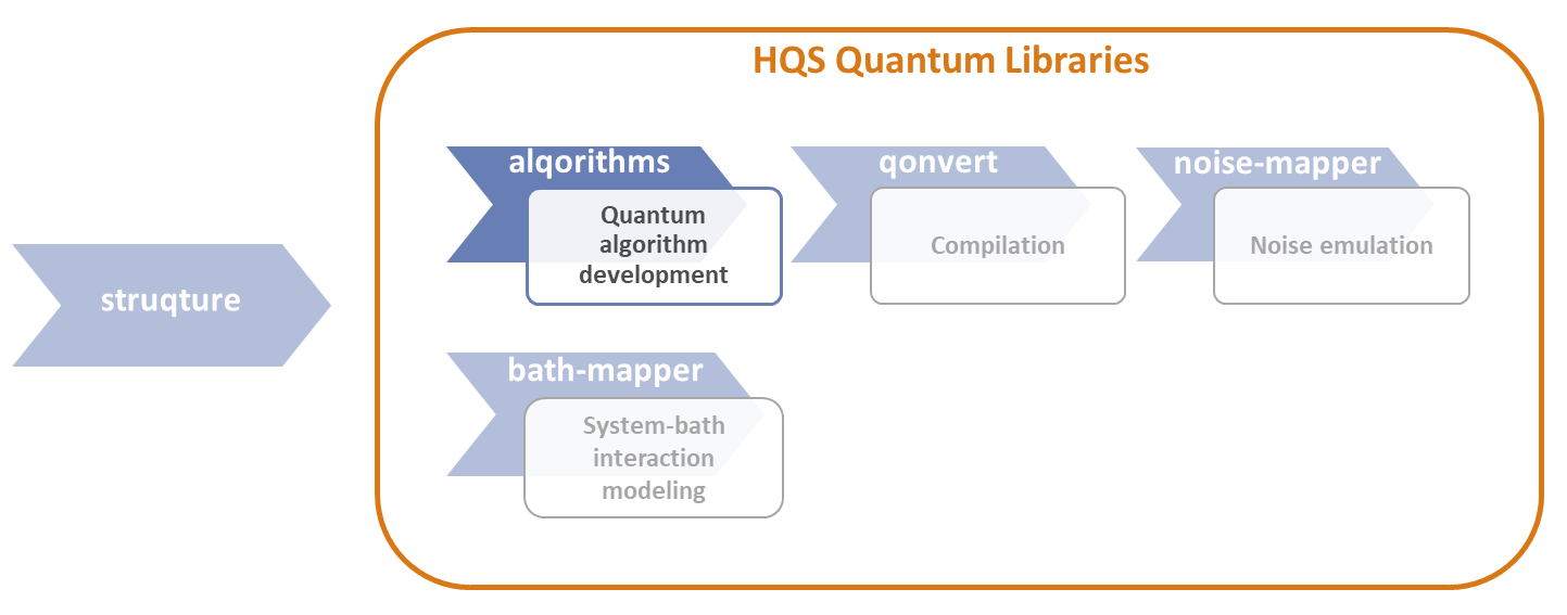
Figure 1: HQS Quantum Libraries - Alqorithms
Applications
Quantum algorithms form the foundation of any software application intended for use on a quantum computer. In the gate-based quantum computing paradigm, these algorithms are implemented as quantum circuits composed of gate operations. Measurements are performed at the end of such circuits to extract computational results. The alqorithms package is a comprehensive toolkit that facilitates these major stages of quantum algorithm development. Its key features include:
- Tools for constructing quantum circuits.
- A collection of algorithms for generating the Trotterized time evolution of quantum systems. These include the ParityBased (CNOT) algorithm, the QSWAP algorithm, and the Mølmer-Sørensen algorithm.
- Circuit-building utilities for diverse measurement schemes.
- Algorithms for computing two-point correlation functions.
Whether the user has a pure system Hamiltonian or a system-bath Hamiltonian, the generated circuits can be executed on a quantum computer using our open-source qoqo-backends.
Getting started
The package can be installed with the following command:
hqstage install py_alqorithms
Please note that the HQS Quantum Libraries are currently only supported on Linux and MacOS.
For an expanded collection of examples please see the examples section.
Features
The currently supported quantum algorithms in the HQS alqorithms package are
- the CNOT algorithm, which assumes qubits with all-to-all connectivity,
- the Mølmer-Sørensen Algorithm, which is similar to the CNOT algorithm but implements a different two-qubit gate,
- and the QSWAP algorithm, which assumes qubits with linear connectivity.
All of these algorithms can take a pure system Hamiltonian or a system-bath Hamiltonian, and the generated circuit can be run on a quantum computer using the HQS open source qoqo-backends.
Furthermore, alqorithms includes tools to create quantum circuits that prepare measurements, which are essential to read out information in quantum computing algorithms. Additionally, the HQS package provides functionalities to perform quantum simulations of two-point correlators in the infinite temperature state. The user can also apply a symmetrization on a spin system to simplify the computation.
The core alqorithms package is written in Rust, and features a Python interface named py-alqorithms. Thus, it combines the performance and memory safety benefits of Rust with the user-friendly accessibility of Python. Rust ensures high-efficiency and reliable execution. The Python interface makes the package usable for a broader audience from the Python's extensive ecosystem, while leveraging the Rust-based core. This setup offers the best of both worlds—high performance at the core and easy integration and prototyping through Python.
The API documentation can be found at the following link:
Available Algorithms
All available algorithms share a common interface. Each algorithm can be initialized with the
desired number_trotter_steps, order (i.e. the order of the trotterization), and the
decomposition_blocks boolean flag. When decomposition_blocks is set to True, the circuit
resulting from each term in the Hamiltonian is wrapped with PragmaStartDecompositionBlock and
PragmaStopDecompositionBlock operations, which are needed for noise
mapping.
Once an instance of the desired algorithm is initialized, a circuit can be constructed with the
create_circuit method, by passing as inputs the Hamiltonian for the time evolution, and the time
parameter. See the Examples section for more details.
Every available algorithm is designed with a specific device connectivity in mind. In order to run a circuit on a device with a particular connectivity graph, additional routing or transpilation steps might be necessary.
CNOT Algorithm
System-Only CNOT Algorithm
The CNOTAlgorithm is used to generate quantum circuits that implement the exponentials of
PauliProducts. It assumes full connectivity between the qubits, or at least that a CNOT gate is
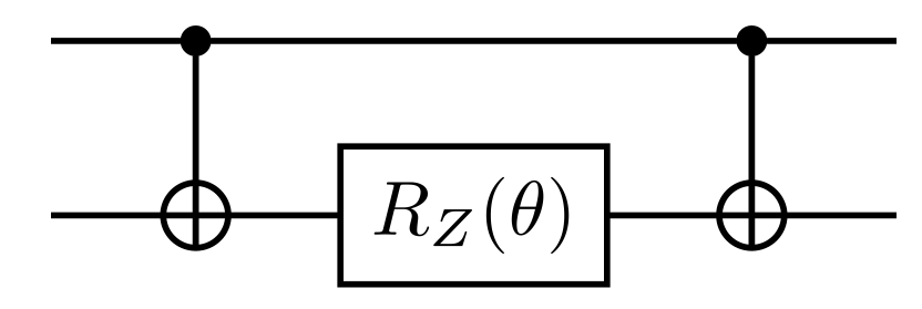
natively available on each pair of qubits. For each term in the PauliProduct, the following
operations are applied:
- The appropriate basis rotation is applied to transform it to the Pauli basis
- A sequence of CNOT gates is applied between each qubits that appear in the Pauli string
- A
RotateZis applied to the last qubit in thePauliProduct - The sequence of CNOTs is applied in reverse
- The basis rotations are undone
For example, the CNOT decomposition for the term is given by the following circuit
and similarly for
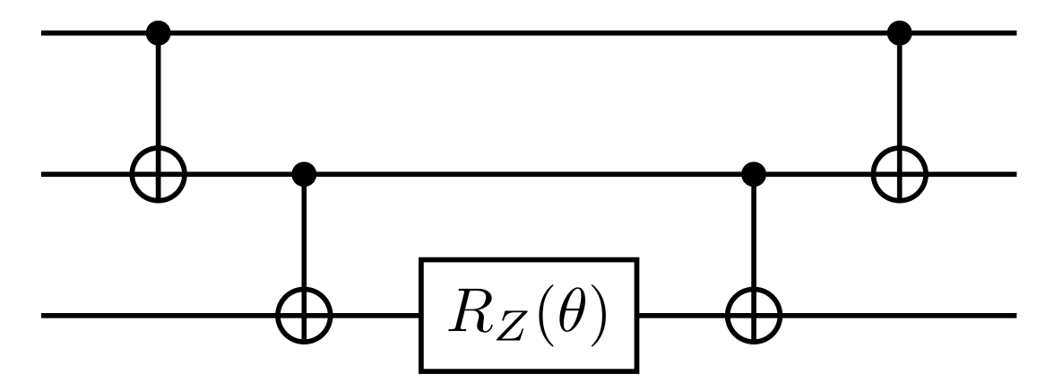
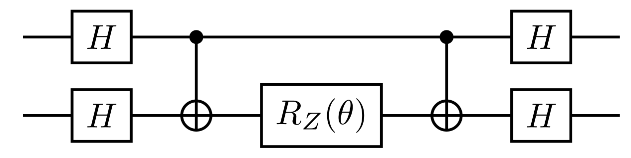
For the term
we need basis rotations with Hadamard gates
System-Bath CNOT Algorithm
The SystemBathCNOTAlgorithm generalizes the CNOTAlgorithm to the case of a spin system coupled
to a spin bath.
The use_bath_as_control boolean flag is used to decide which one between the system qubit and the
bath qubit involved in a two-qubit interaction term should be the control, and which should be the
target, and therefore also on which of the two the single qubit rotation is applied.
All system-only or bath-only terms are implemented using the CNOTAlgorithm, while the two-qubit
interaction terms between system and bath are implemented with the following logic:
- If the bath operator is Pauli , then the system basis is rotated to the Pauli basis,
and CNOTs are added as in the
CNOTAlgorithm, with the single-qubit rotation involved beingRotateX(applied on the bath qubit or the system qubit depending onuse_bath_as_control). - If the bath operator is not Pauli , the same logic as the
CNOTAlgorithmis used, again withuse_bath_as_controldeciding on which qubit theRotateZis applied.
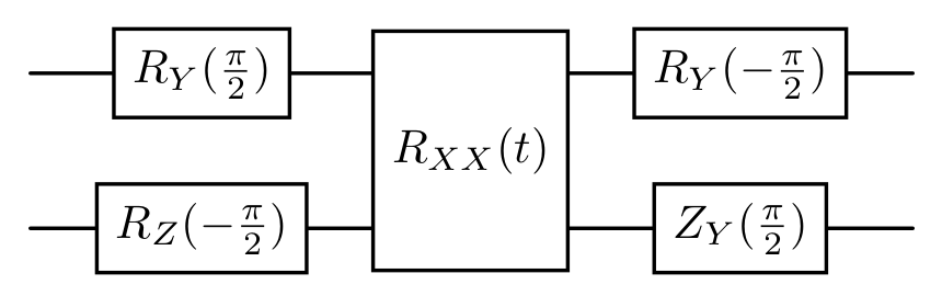
Mølmer-Sørensen Algorithm
The VariableMSXXAlgorithm is similar to the CNOTAlgorithm, and only differs
in the implementation of the two-qubit gates. While the CNOTAlgorithm treats two-qubit and
multi-qubit gates equally, the VariableMSXXAlgorithm implements two-qubit gates using the
VariableMSXX gate (i.e. ) and basis rotations if needed.
For example, the term is implemented as
QSWAP Algorithms
System-Only QSWAP Algorithms
The QSWAPAlgorithm and QSWAPMSAlgorithm implement the swapping algorithm presented in this
paper to simulate the (second order) trotterized time evolution
of a system of qubits on a device with linear connectivity. They only differ in the way they
implement multi-qubit gates: the QSWAPAlgorithm uses the CNOTAlgorithm,
while QSWAPMSAlgorithm uses the VariableMSXXAlgorithm.
In order to implement two-qubit gates between qubits that are not nearest neighbors, the algorithm uses a SWAP network to shuffle the order of the logical qubits, so that each pair of logical qubits is encoded in a pair of nearest neighboring physical qubits at least once during the swapping procedure.
The SWAP network alternates even and odd layers of SWAP gates
where the even layers apply the SWAPs to the even indices, and the odd layers to the odd indices. Indicating by a dash the (logical) qubits being swapped, we have
Even layer: Odd layer:
This swapping procedure shuffles the pairs that are found next to each other at every layer. After layers of this external swap network, the logical qubits recover their original ordering. During the swapping, all logical qubits are found next to each other at least once, and the relevant interactions can be implemented.
System-Bath QSWAP Algorithms
Similar to the system-only algorithms, the SystemBathQSWAPAlgorithm and the
SystemBathQSWAPMSAlgorithm implement the swapping procedure described above for a spin system
coupled to a non-interacting spin bath, and they only differ in the multi-qubit gates implementation.
The connectivity graph between the qubits consists of three parallel linear chains, with the corresponding qubits from each chain coupled with each other. The central chain represents the system qubits, while the two external chains the bath qubits. Since the bath is non-interacting, only the system qubits are swapped.
NMR Algorithm
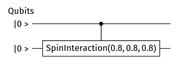
The NMRHamiltonianAlgorithm constructs quantum circuits for Hamiltonians containing XX, YY, and ZZ two-qubit interaction terms. This yields shallower circuits with fewer two-qubit gates than a CNOT-based decomposition, and avoids the SWAPs generated in a QSWAP-based decomposition. It uses the SpinInteraction gate, which Qonvert can decompose more efficiently than the gate sequences produced by the CNOTAlgorithm. This is particularly useful for simulating the second-order Trotterized time evolution of NMR Hamiltonians on devices with linear connectivity, since such Hamiltonians predominantly comprise XX, YY, and ZZ interactions.
The SpinInteraction gate represents a generalized, anisotropic XYZ Heisenberg interaction between spins. It applies the following unitary to qubits t and c:
Example
Here is an example with a two-spin Hamiltonian:
hamiltonian = spins.PauliHamiltonian()

for i in range(number_spins):
    for j in range(i + 1, number_spins):
        for op in ["X", "Y", "Z"]:
            hamiltonian.set(f"{i}{op}{j}{op}", 0.4)
PauliHamiltonian{
0X1X: 4e-1,
0Y1Y: 4e-1,
0Z1Z: 4e-1,
}
When using the NMRHamiltonianAlgorithm to create the trotterized time evolution of the Hamiltonian we obtain the following circuit:
unitary = py_alqorithms.NMRHamiltonianAlgorithm(number_trotter_steps=1).order(1)
circuit = unitary.create_circuit(hamiltonian, 2.0)
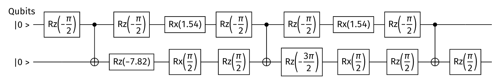
This time-evolution circuit can then be compiled for a specific device (here containing RotateZ, RotateX, and CNOT gates) using qonvert, resulting in a circuit with 2 two-qubit gates:
With the CNOTAlgorithm, on the other hand, we obtain the following time-evolution circuit:
unitary = py_alqorithms.CNOTAlgorithm(number_trotter_steps=1).order(1)
circuit = unitary.create_circuit(hamiltonian, 2.0)
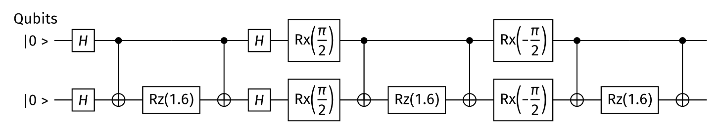
Running the qonvert compilation for the same device, we obtain a circuit with 6 two-qubit gates:
Limitations
While this algorithm is the best choice for these kinds of Hamiltonians, using it with a Hamiltonian with a term other than XX, YY or ZZ will result in an error.
Measurement Circuits
alqorithms includes tools to create circuits that prepare measurements. The convention in
gate-based quantum computing is that projective measurements of a quantum register happen by default
in the Pauli Z basis. In other words, it is only possible to directly measure operators of the form
where .
In order to measure arbitrary Pauli strings, we need to append a measurement circuit at the end of our circuit to rotate the basis of the quantum register so that the standard measurement in the Pauli Z basis effectively corresponds to a measurement of the desired Pauli string.
Creating a single measurement circuit
In order to measure an arbitrary Pauli string , where , we need to apply single-qubit rotations to the qubits in the quantum register in order to rotate them from the Z basis to the eigenbasis of the corresponding entry in the Pauli string that we want to measure.
We can even measure multiple Pauli strings with the same measurement circuit, provided that they commute with each other. Two Pauli strings commute with each other if, for each qubit in the quantum register, both PauliProducts have either the same PauliOperator (X, Y, Z) or at least one has the identity operator. Such Pauli strings are compatible because they can be diagonalized simultaneously, which means that we can use a single measurement circuit to rotate the quantum register into their common eigenbasis.
In alqorithms, a measurement circuit can be created with the single_measurement_circuit
function, as follows.
from struqture_py import PauliProduct
from hqs_quantum_libraries.alqorithms import single_measurement_circuit

# These PauliProducts are compatible
pp1 = PauliProduct.from_string("0X2Y3Z")
pp2 = PauliProduct.from_string("0X1Z")
pp3 = PauliProduct.from_string("2Y3Z")

meas_circuit = single_measurement_circuit([pp1, pp2, pp3], "ro", False, 4)
Creating a measurement for an observable
If we want to measure an arbitrary observable, represented in struqture as a linear combination of
PauliProducts, in general, the Pauli products will not all be compatible with each other. We will
then need multiple measurement circuits that we'll use to perform separate measurements for each set
of compatible PauliProducts. For this, we can use the function measure_spin_operator (or
measure_spin_operator_map if we have a list of operators to measure), returning a qoqo
PauliZProduct, an object that collects all the information needed to perform the separated
measurements and post-process the measurement results into the expectation value of the observable.
It can be used as follows
from qoqo import Circuit
from qoqo import Circuit
from qoqo.operations import RotateY
from struqture_py import PauliProduct, PauliOperator
from hqs_quantum_libraries.alqorithms import measure_spin_operator

number_measurements = 10
number_qubits = 5
# whether to undo the basis rotation after the measurement circuit
undo_basis_rotation = False

# Prepare the base circuit after which to measure the observable
constant_circuit = Circuit()
for qubit in range(number_qubits):
    constant_circuit += RotateY(qubit, 0.5)

pauli_products = [
  # First set of compatible PauliProducts
  "0X2Y3Z",
  "0X1Z",
  "2Y3Z",
  # Second set of compatible PauliProducts
  "0Z2Z3X",
  "0Z3X",
  "1Y2Z",
]

op = PauliOperator()
for pp in pauli_products:
    op.set(pp, 1.0)

measurement = measure_spin_operator(
    op,
    constant_circuit,
    "my_op",
    undo_basis_rotation,
    number_measurements
)
This measurement can then be used in a QuantumProgram as follows
from qoqo_quest import Backend
from qoqo import QuantumProgram

backend = Backend(number_qubits)
qp = QuantumProgram(measurement, [])
qp.run(backend, None)
Similarly we can create cheated measurements (CheatedPauliZProduct) using the function
measure_spin_operator_map_cheated.
Correlators
alqorithms provides the class InfiniteTemperatureCorrelator to create qoqo QuantumPrograms to
perform quantum simulations of two-point correlators in the infinite temperature state.
Infinite Temperature State Preparation
We want to measure correlators of the form with respect to the infinite-temperature state, represented by the maximally-mixed density matrix
There are different ways to achieve this. The default initialization is all_initial_states, which
measures the infinite temperature operator by running the correlation measurement over all
possible time-evolved eigenstates of the operator. With this option, the number of
circuits and measurements scales exponentially with the number of qubits. It has, however, the least
requirements for the quantum computer. Other ways to prepare the infinite-temperature state can
require active-reset or mid-circuit measurement operations.
The other available initializations are:
-
measurement: Uses an initialization that prepares the infinite-temperature state by measuring after a Hadamard gate. This can only be applied when the number of measurements is comparable to the dimension of the Hilbert space of the system. The sequence is: Hadamard on all qubits -> Measure -> Rotate into basis -> Measure -> Rotate back from basis. It is recommended to only use this on an experimental basis. -
dephasing: Uses an initialization that prepares the infinite-temperature state by dephasing after applying Hadamard gates. This can only be applied when the number of measurements is comparable to where is the number of qubits the operator acts on. The sequence is: Hadamard on all qubits -> Let system dephase -> Rotate into basis -> Measure -> Rotate back from basis. It is recommended to only use this on an experimental basis. -
local_operator_measurement: Uses an initialisation that prepares the infinite-temperature state by applying Hadamard gates and using the measurement that is normally necessary to extract the correlator with the correlation operator. This can only be applied when the operator is a sum of local operators and the number of measurements is comparable to the dimension of the Hilbert space of the system. The sequence is: Hadamard on all qubits -> Measure -> Rotate back from basis. It is recommended to only use this on an experimental basis. -
active_reset: Uses an initialisation that prepares the infinite-temperature state by dephasing after applying Hadamard gates. Assumes the operator only acts on one qubitq. Actively resets the qubit the operator is acting on and adds two measurement circuits:- One where the qubit is set to 0 and the output of a virtual qubit is set to zero
- One where the qubit is set to 1 and the output of a virtual qubit is set to zero
This avoids measuring inside the circuit which is more efficient. This can only be applied when the operator is a sum of local operators and the number of measurements is comparable to the dimension of the Hilbert space of the system. The sequence is: Hadamard on all qubits -> ActiveReset on
q-> Two Circuits: One whereqis 0 one whereqis 1 -> Rotate back from basis. -
all_initial_states: Measures the infinite temperature operator by running the Correlation measurement over all possible initial eigenstates of the right operator in the trace. For example if B = σ^z, the trace is computed over the basis (|000...>, |001...>, ..., |010...>, ..., |011...>, ...) With this option the number of circuits and measurements scales exponentially with the number of qubits. -
positive_magnetization: Measures the infinite temperature operator by running the Correlation measurement over the subset of the initial eigenstates of the right operator in the trace that have positive magnetization. -
random_states: Measures the infinite temperature operator by running the Correlation measurement over a random subset of the initial eigenstates of the right operator in the trace.
Usage
Once initialized, the class InfiniteTemperatureCorrelator provides three methods to compute the
desired correlator:
time_correlation_measurement: Run the measurement for a single correlator.time_correlation_measurement_multiple_left: Run the measurement for a list of correlators that have different left operators . It works liketime_correlation_measurement, but a list of left operators is passed as input instead of a single operator. The outputQuantumProgramhas a symbolic parameter for the evolution time.time_correlation_measurement_multiple_left_fixed_timestep: Similar to the method above, but allows to pass a fixed trotter timestep. The outputQuantumProgramhas a symbolic parameter for the number of trotter steps.
The following example in Python shows how to initialize the InfiniteTemperatureCorrelator class
and use it to compute the correlator .
from hqs_quantum_libraries.alqorithms import InfiniteTemperatureCorrelator
from struqture_py import PauliOperator, PauliHamiltonian
from qoqo import QuantumProgram

number_spins = 3

# Set up Hamiltonian for time evolution
hamiltonian = PauliHamiltonian()
for i in range(number_spins-1):
    hamiltonian.add_operator_product(f"{i}X{i + 1}X", 1.0)
for i in range(number_spins):
    hamiltonian.add_operator_product(f"{i}Z", 1.0)
print(f"Hamiltonian: \n{hamiltonian}\n")


# Define right and left operators to correlate
left_op = PauliOperator()
left_op.add_operator_product("0Y", 1.0)
print(f"Left operator: \n{left_op}\n")

right_op = PauliOperator()
right_op.add_operator_product("1Z", 1.0)
print(f"Right operator: \n{right_op}\n")

# Initialize correlator class
correlator = InfiniteTemperatureCorrelator(number_trottersteps=100)
correlator.algorithm = "ParityBased"
correlator.number_measurements = 10000
correlator.initialisation = "all_initial_states"
print("Correlator: ", correlator)

# Construct quantum program
measurement = correlator.time_correlation_measurement(left_op, hamiltonian, right_op)
program = QuantumProgram(measurement, [])
Symmetrization
The py_alqorithms.symmetrization module provides functions to symmetrize a spin system by
conjugating the Hamiltonian with Pauli operators.
Pure Spin System
For pure systems, the following two functions are provided:
-
create_symmetrized_spin_circuit: Creates a quantum circuit implementing the trotterized time evolution with the Hamiltonianwhere is the input spin Hamiltonian.
-
apply_symmetrization_spins: Similar to the function above, but additionally applies aPauliXgate to every qubit to switch the definition of and , both before and after the circuit implementing the trotterized time evolution with the symmetrized Hamiltonian.
Example
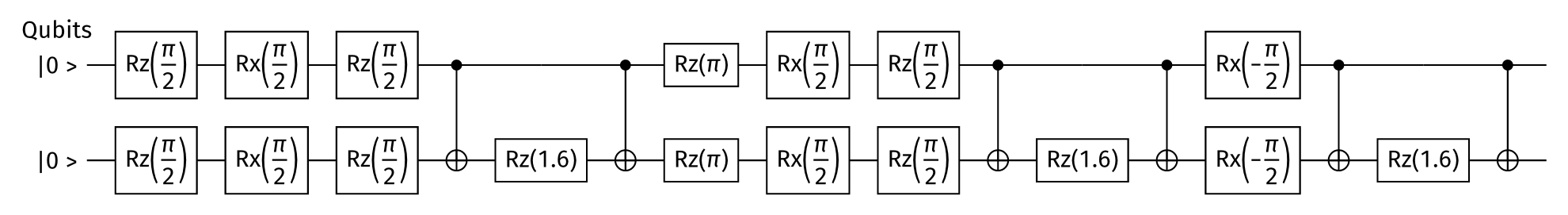
A minimal example describing the use of apply_symmetrization_spins function.
The hamiltonian is given by
Figure 1 illustrates the time evolution circuit of with two trotter steps.
from struqture_py.spins import PauliHamiltonian, PauliProduct

# Parameters
algorithm = "ParityBased"
trotterization_order = 1
number_trottersteps = 2
time = 5.0

# Initializing spin hamiltonian
hamiltonian = PauliHamiltonian()
hamiltonian.add_operator_product(PauliProduct().z(0), 0.5)
hamiltonian.add_operator_product(PauliProduct().z(1), 1.0)

# Symmetrizing spin circuit
circuit = hqs_quantum_libraries.alqorithms.apply_symmetrization_spins(
    algorithm,
    hamiltonian,
    trotterization_order,
    number_trottersteps,
    time
)
 Figure 1: Trotterized time evolution of spin hamiltonian
System-Bath
For system-bath algorithms, the following functions are provided:
create_symmetrized_system_bath_circuit: Similar tocreate_symmetrized_spin_circuit, only applying the transformation to the system qubits. Together with the resulting circuit created by the selected algorithm, it also returns the list of qubits that constitute the system.apply_symmetrization_system_bath- Similar toapply_symmetrization_spins, only applying the transformation to system qubits.
Example
A minimal example describing the symmetrization of a system-bath circuit. The hamiltonian is given by
Figure 2 illustrates a single trotter step time evolution of the system-bath hamiltonian.
from struqture_py.spins import PauliProduct
from struqture_py.mixed_systems import MixedHamiltonian, HermitianMixedProduct

# Parameters
algorithm = "ParityBased"
number_trottersteps = 1
time = 5.0
remapping = ([0, 1], [2, 3, 4, 5], None)
use_bath_as_control = False

# Initializing the system bath hamiltonian
hamiltonian = MixedHamiltonian(2, 0, 0)
hamiltonian.add_operator_product(
    HermitianMixedProduct(
        [PauliProduct().z(0), PauliProduct()],
        [],
        []
    ),
    0.5
)

hamiltonian.add_operator_product(
    HermitianMixedProduct(
        [PauliProduct().x(1), PauliProduct().x(0)],
        [],
        []
    ),
    0.5
)
hamiltonian.add_operator_product(
    HermitianMixedProduct(
        [PauliProduct(), PauliProduct().z(1)],
        [],
        []
    ),
    1.0
)

# Symmetrizing system-bath circuit
circuit = hqs_quantum_libraries.alqorithms.apply_symmetrization_system_bath(
    algorithm,
    hamiltonian,
    number_trottersteps,
    time,
    use_bath_as_control,
    remapping
)
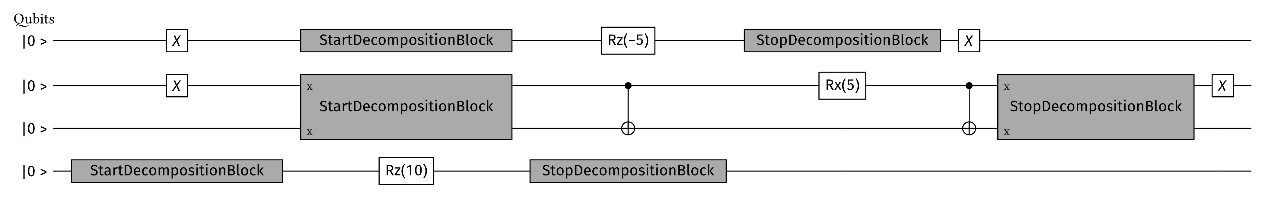 Figure 2: Trotterized time evolution of system-bath hamiltonian
Examples
CNOTAlgorithm
from struqture_py.spins import PauliProduct, PauliHamiltonian
from hqs_quantum_libraries.alqorithms import CNOTAlgorithm

# create Hamiltonian
hamiltonian = PauliHamiltonian()
hamiltonian.set("0X2Y", 0.5)
hamiltonian.set("1Z3X", 1.5)
hamiltonian.set("0Z", 1.0)
hamiltonian.set("2X", 1.0)

# create algorithm (here with second order trotterization)
alg = CNOTAlgorithm(number_trotter_steps=10).decomposition_blocks(True).order(2)
time = 3.0

# create circuit
circuit = alg.create_circuit(hamiltonian, time)
VariableMSXXAlgorithm
from struqture_py.spins import PauliProduct, PauliHamiltonian
from hqs_quantum_libraries.alqorithms import VariableMSXXAlgorithm

# create Hamiltonian
hamiltonian = PauliHamiltonian()
hamiltonian.set("0X2Y", 0.5)
hamiltonian.set("1Z3X", 1.5)
hamiltonian.set("0Z", 1.0)
hamiltonian.set("2X", 1.0)

# create algorithm
alg = VariableMSXXAlgorithm(number_trotter_steps=10).decomposition_blocks(True)
time = 3.0

# create circuit
circuit = alg.create_circuit(hamiltonian, time)
QSWAPAlgorithm
from struqture_py.spins import PauliProduct, PauliHamiltonian
from hqs_quantum_libraries.alqorithms import QSWAPAlgorithm

# create Hamiltonian
hamiltonian = PauliHamiltonian()
hamiltonian.set("0X3Y", 0.5)
hamiltonian.set("0Z2X", 1.5)
hamiltonian.set("0Z1Y", 1.0)
hamiltonian.set("2X", 1.0)
hamiltonian.set("1Z", 1.0)

# create algorithm
alg = QSWAPAlgorithm(number_trotter_steps=10).decomposition_blocks(True)
time = 3.0

# create circuit
circuit = alg.create_circuit(hamiltonian, time)