Elastic constants

The theory in this section relates to the functions under the elastic module.

Introduction

Elastic constants measure the proportionality between strain and stress in a crystal, provided that the strain is not so large as to violate Hooke’s law.

—D. A. Papaconstantopolous

As noted by Papconstantopolous, the elastic constants may be considered a three-dimensional generalisation of Hooke’s law, where put simply, the restoring force \(F\), is proportional to the so-called spring constant \(k\) times the displacement \(dx\) so long as the material is within the “elastic region”. Elastic constants can be used for several purposes, they provide information about the speed of sound in materials, they tell how strong a material is and can give important information as to whether the material is structurally stable. They also (and most interestingly for us) can be used to predict equilibrium lattice distortions in heterostructures and estimate stress (strain) given an input strain (stress). In this work we will be discussing the methodologies for computing elastic constants using Ab Initio techniques.

Discussion

For the following we will be using the Voigt notation to simplify higher order tensors to lower order ones. In particular reduction of the fourth-order elastic stiffness tensor and second order stress/strain tensors allows us to reduce the entire elasticity problem to a linear equation. Derivation of the elastic tensor is quite lengthy and will not be discussed here, instead we focus specifically on the stress and strain matrices \(\sigma\) and \(\epsilon\), respectively. Most generally they may be written as:

\[\begin{split}\sigma = \left[ \begin{array}{ccc} \sigma_{xx} & \sigma_{xy} & \sigma_{xz} \\ \sigma_{yx} & \sigma_{yy} & \sigma_{yz} \\ \sigma_{zx} & \sigma_{zy} & \sigma_{zz} \end{array} \right], \quad \epsilon = \left[ \begin{array}{ccc} \epsilon_{xx} & \epsilon_{xy} & \epsilon_{xz} \\ \epsilon_{yx} & \epsilon_{yy} & \epsilon_{yz} \\ \epsilon_{zx} & \epsilon_{zy} & \epsilon_{zz} \end{array} \right].\end{split}\]

For these works it is important to define what the directions \(x,y,z\) mean. In general they define any complete coordinate system (basis vectors) of a three-dimensional space. In practice, they refer more specifically to the first, second and third components of the lattice vectors of a crystal in its standard (primitive) representation, so that we may unambiguously exploit its symmetry later in this document. It is important that these lattice vectors be described in their standard representation as the deformation matrix is not invariant with respect to rotation. The elastic constants tensor may be posthoc rotated to the symmetric frame by using a transformation matrix but this requires that the full, rather than symmetry-reduced, tensor be computed. It is therefore recommended that for whatever crystal used that you output its standard primitive form by spglib.

Resuming our discussion, regardless of orientation chosen, under Voigt notation these matrices are assumed symmetric. Therefore in the mapping, we make sure to take only the symmetric part, for stress we use:

\[\begin{split}\begin{gathered} \sigma_{1} = \sigma_{xx}, \quad \sigma_{2} = \sigma_{yy}, \quad \sigma_{3} = \sigma_{zz}, \nonumber \\ 2\sigma_{4} = \sigma_{yz}+\sigma_{zy}, \quad 2\sigma_{5} = \sigma_{xz} + \sigma_{zx}, \quad 2\sigma_{6} = \sigma_{xy} + \sigma_{yx}, \end{gathered}\end{split}\]

or explicitly:

\[\begin{aligned} \tilde{\sigma} \ = \ \left( \sigma_{xx}, \quad \sigma_{yy}, \quad \sigma_{zz}, \quad \frac{\sigma_{yz}+\sigma_{zy}}{2}, \quad \frac{\sigma_{xz}+\sigma_{zx}}{2}, \quad \frac{\sigma_{xy}+\sigma_{yx}}{2} \right), \end{aligned}\]

this conversion may be found in convert_stress_in_matrix_form_to_voigt_form(), whereas for strain (paying special attention the last three components) the mapping is:

\[\begin{split}\begin{gathered} \epsilon_{1} = \epsilon_{xx}, \quad \epsilon_{2} = \epsilon_{yy}, \quad \epsilon_{3} = \epsilon_{zz}, \nonumber \\ \epsilon_{4} = \epsilon_{yz}+\epsilon_{zy}, \quad \epsilon_{5} = \epsilon_{xz} + \epsilon_{zx}, \quad \epsilon_{6} = \epsilon_{xy} + \epsilon_{yx}, \end{gathered}\end{split}\]

or explicitly:

\[\begin{aligned} \tilde{\epsilon} \ = \ \left( \epsilon_{xx}, \quad \epsilon_{yy}, \quad \epsilon_{zz}, \quad \epsilon_{yz}+\epsilon_{zy}, \quad \epsilon_{xz}+\epsilon_{zx}, \quad \epsilon_{xy}+\epsilon_{yx} \right), \end{aligned}\]

this conversion may be found in convert_strain_in_matrix_form_to_voigt_form().

We may then reverse the mapping to give our second-order tensors:

\[\begin{split}\sigma = \left[ \begin{array}{ccc} \sigma_{1} & \sigma_{6} & \sigma_{5} \\ & \sigma_{2} & \sigma_{4} \\ \text{sym} & & \sigma_{3} \end{array} \right], \quad \epsilon = \left[ \begin{array}{ccc} \epsilon_{1} & \epsilon_{6}/2 & \epsilon_{5}/2 \\ & \epsilon_{2} & \epsilon_{4}/2 \\ \text{sym} & & \epsilon_{3} \end{array} \right]\end{split}\]

where the asymmetric components have been explicitly discarded, these functions are found under convert_stress_in_voigt_form_to_matrix_form() and convert_strain_in_voigt_form_to_matrix_form() respectively.

After mapping to Voigt notation, the most general stress-strain relation is thence:

\[\begin{split}\left[ \begin{array}{c} \sigma_{1} \\ \sigma_{2} \\ \sigma_{3} \\ \sigma_{4} \\ \sigma_{5} \\ \sigma_{6} \end{array} \right] = \left[ \begin{array}{c} \sigma^{(0)}_{1} \\ \sigma^{(0)}_{2} \\ \sigma^{(0)}_{3} \\ \sigma^{(0)}_{4} \\ \sigma^{(0)}_{5} \\ \sigma^{(0)}_{6} \end{array} \right] + \left[\begin{array}{cccccc} C_{11} & C_{12} & C_{13} & C_{14} & C_{15} & C_{16}\\ & C_{22} & C_{23} & C_{24} & C_{25} & C_{26}\\ & & C_{33} & C_{34} & C_{35} & C_{36}\\ & & & C_{44} & C_{45} & C_{46}\\ & & & & C_{55} & C_{56}\\ \text{sym} & & & & & C_{66} \end{array}\right] \left[ \begin{array}{c} \epsilon_{1} \\ \epsilon_{2} \\ \epsilon_{3} \\ \epsilon_{4} \\ \epsilon_{5} \\ \epsilon_{6} \end{array} \right]\end{split}\]

where \(\sigma^{0}_i\) are the strains of the reference system, ideally zero. More succinctly, this may be written as:

(1)\[ \sigma_i = \sigma_i^{0} + \sum_{j=1}^{6} C_{ij} \epsilon_j + \mathcal{O}(\epsilon^2)\]

Similarly, the total energy of the system is computed using a Taylor expansion in \(\epsilon\) up to second order:

(2)\[ E = E_0 + V_0 \left( \sum_{i=1}^{6} \sigma_{i}^{(0)} \epsilon_{i} + \frac{1}{2} \sum_{i,j=1}^{6} C_{ij} \epsilon_{i} \epsilon_{j} \right) + \mathcal{O}(\epsilon^3)\]

where \(E_0\) and \(V_0\) are the total energy and volume of the reference system respectively. Naturally, if the system is relaxed the linear stress terms vanish. Now that we have covered the very basics of elastic constants, let’s explore how we compute them.

Computing elastic constants

There are two main strategies for computing the elastic constants computationally. The first, known as the “Energy approach”, is based off of the energy changes one observes due to deforming the crystal using (2). The second, known as the “Stress theorem” is based on varying the strain of the crystal and monitoring the changes in the stress via (1). Both have their strengths and weaknesses as we will discuss below. To make the discussion more accessible, we demonstrate both methods using a model cubic system. Under the symmetries of a cubic system, the elastic tensor reduces to:

\[\begin{split}C_\text{cubic} = \left[\begin{array}{cccccc} C_{11} & C_{12} & C_{12} & 0 & 0 & 0 \\ C_{12} & C_{11} & C_{12} & 0 & 0 & 0 \\ C_{12} & C_{12} & C_{11} & 0 & 0 & 0 \\ 0 & 0 & 0 & C_{44} & 0 & 0 \\ 0 & 0 & 0 & 0 & C_{44} & 0 \\ 0 & 0 & 0 & 0 & 0 & C_{44} \end{array}\right],\end{split}\]

containing only 3 independent elastic constants.

Aside: Symmetry

Certain methods such as ULICS [ULICS] use a set of dense vectors to sample as much of phase space as possible by coupling as many degrees of freedom as possible. This method though sensible in its goal of coupling degrees of freedom falls short when the symmetry of the problem is taken into account. Consider for instance a square lattice, the Irreducible Brillouin Zone (IBZ) is reduced to 1/8th the size of the full Brillouin Zone (BZ). If the symmetry is broken, and that all other properties converge just as quickly, this would be at least an \(8\times\) slowdown; one could compute 7 more highly symmetric evaluations in the time it takes to compute one asymmetric one. For this reason we use a set of highly symmetric vectors based off of OHESS (Liu), IRelast (Jamal et al.) and VASP (Saxe et al.) to maximally sample our space in the fewest and fastest vectors possible.

Energy-based

To compute properties efficiently using the energy approach we use the basis sets detailed in the papers by Jamal et al. [Jamal2014], [Jamal2018], where the authors optimized their vector choices to preserve the symmetry as much as possible and (interestingly) simultaneously constraining them to conserve volume where possible, where this second correction is most important for high-pressure systems due to the nature of the energy expansion in P and V. By preserving symmetry we can use fewer (\(k\)-point) evaluations to achieve the same results at a fraction of the cost.

As energy converges much more quickly than other properties of Ab Initio simulations this method is numerically well-behaved but suffers from one major drawback; only one degree of freedom may be sampled as the energy method is a many-to-one operation. Nevertheless, it is both a useful method especially in the context of systems where the stress tensor (and the forces on atoms) cannot be computed. In such a case only the so-called “clamped” elastic constants can be computed as one cannot relax the atomic positions, or if say a method like GW, they are relaxed before applying the correction.

We break this method up into three parts, volumetric expansion, orthorhombic deformation and monoclinic deformation.

Volumetric expansion

For volumetric expansion, the strain tensor is given by:

\[\begin{split}\epsilon_\text{cubic} = \left( \begin{array}{ccc} \varepsilon & 0 & 0 \\ 0 & \varepsilon & 0 \\ 0 & 0 & \varepsilon \end{array} \right)\end{split}\]

where \(\varepsilon\) is used to denote a general strain “value" rather than the strain tensor. This expansion completely preserves the symmetry of the underlying lattice but as the name suggests, does not (and cannot) preserve volume by some correction like our other strain types. Using this strain tensor results in:

(3)\[E \approx E_0 + V_0 (\sigma^{(0)}_1 + \sigma^{(0)}_2 + \sigma^{(0)}_3)\varepsilon + \frac{3 V_0}{2}(C_{11} + 2 C_{12})\varepsilon^2 + \mathcal{O}(\varepsilon^3)\]

where (for cubic crystals) \((C_{11}+2C_{12})/3\) is known as the Bulk Modulus, B. With this one can extract the bulk modulus from the second derivative using either finite difference, linear regression or by fitting an equation of state. In particular, the Birch-Murnaghan equation of state is very useful as it is derived from first principles and works for both high and low pressure limits, something which many phenomenological or perturbative fits do not. In terms of the pressure, it is given by:

\[P(V) = \frac{3 B_0}{2} \left[ \left(\frac{V_0}{V}\right)^{\frac{7}{3}} - \left(\frac{V_0}{V}\right)^{\frac{5}{3}}\right] \left\lbrace 1 + \frac{3}{4}\left(B_0^\prime - 4\right) \left[\left(\frac{V_0}{V}\right)^{\frac{2}{3}} - 1\right] \right\rbrace\]

where \(B_0\), \(B^\prime_0\) and \(V_0\) are the zero pressure bulk modulus, bulk modulus derivative (w.r.t. pressure) and volume respectively. For our purposes we the internal energy (its integral) given by:

(4)\[\Delta E(V) = \frac{9 V_0 B_0}{16} \left\lbrace \left[ \left(\frac{V_0}{V}\right)^{\frac{2}{3}} - 1 \right]^3 B_0^\prime + \left[\left(\frac{V_0}{V}\right)^{\frac{2}{3}} - 1 \right]^2 \left[6 - 4 \left(\frac{V_0}{V}\right)^{\frac{2}{3}}\right] \right\rbrace\]

we also use this method in our workflow to attain accurate estimates for the equilibrium lattice constant. To see why this is so helpful, first we take the Taylor series of (4) we arrive at:

\[\Delta E(V) \approx \frac{V_0 B_0}{2} \left( \frac{V}{V_0} - 1 \right)^2\]

which is the simplest expression that gives \(B_0 = \partial^2 E(V)/\partial V^2\) (everywhere) this allows us to see where higher order effects come into play by directly comparing against (4). Then, noting that volumetric expansion \(V = V_0 (1+\epsilon)^3\), we make another expansion in small \(\epsilon\) to see:

\[\Delta E(V) \ \approx \ \frac{V_0 B_0}{2} \left(\frac{V_0 (1+\varepsilon)^3}{V_0} - 1 \right)^2 \ \stackrel{\varepsilon \rightarrow 0}{\approx} \ \frac{9 V_0 B_0 \varepsilon^2}{2},\]

and can be seen to be equivalent to (3), thus fitting the Birch-Murnaghan equation of state (which supports high/low pressure solids without or without nonlinear corrections) with least squares gives us a useful estimate where our energy scales act perturbatively, obtain a Bulk modulus value and get a reasonable lattice parameter estimate all in one go.

Orthorhombic deformation

Orthorhombic deformation, as the name suggests, contracts one dimension while expanding another, it is given by:

\[\begin{split}\epsilon_\text{ortho} = \left( \begin{array}{ccc} \varepsilon & 0 & 0 \\ 0 & -\varepsilon & 0 \\ 0 & 0 & \varepsilon^2/(1-\varepsilon^2) \end{array} \right)\end{split}\]

where the (roughly) quadratic correction \(\varepsilon^2/(1-\varepsilon^2)\) component to the third dimension leaves the total volume unchanged (though it will introduce an \(\varepsilon^4\) correction in the total energy, which is subsumed into the overall big O error). Neglecting the component arising from the third dimension, its energy expansion is given by:

\[\begin{aligned} E &\approx E_0 + (\sigma^{(0)}_1 - \sigma^{(0)}_2)\varepsilon + V_0(C_{11}-C_{12})\varepsilon^2 + \mathcal{O}(\varepsilon^3) \end{aligned}\]

where (for cubic crystals) \((C_{11}-C_{12})/2\) is the so-called shear modulus \(C^\prime\). One then computes this using finite differences or linear regression.

Monoclinic deformation

The last deformation type is monoclinic, which unfortunately breaks most of the symmetry in a cubic lattice. It is given by:

\[\begin{split}\epsilon_\text{mono} = \left( \begin{array}{ccc} 0 & \varepsilon & 0 \\ \varepsilon & 0 & 0 \\ 0 & 0 & \varepsilon^2/(1-\varepsilon^2) \end{array} \right)\end{split}\]

where once again the \(\varepsilon^2/(1-\varepsilon^2)\) term in the third dimension is to keep the total volume constant. Its energy expansion (ignoring the components in the third dimension) is given by:

\[E \approx E_0 + \sigma^{(0)}_4\varepsilon + \frac{V_0}{2}(C_{44})\varepsilon^2 + \mathcal{O}(\varepsilon^3)\]

One then computes this using finite differences or linear regression. \(C_{44}\) is related to the so-called anisotropy factor or zener ratio:

\[a_r = \frac{2 C_{44}}{C_{11}-C_{12}},\]

which is unity for isotropic materials.

Stress-based

As before, the eponymous stress-based method calculates the elastic constants by exploiting the many-to-many nature of the stress/strain relations. In order to efficiently and expediently calculate the properties of these crystals we use the Optimized High-Efficiency Strain-matrix Set (OHESS) [OHESS2020] strain sets which have been chosen to maximize both the symmetry and the number of degrees of freedom sampled in one evaluation.

In this example, the OHESS vector is able to sample all three elastic constants of a cubic crystal can be computed using only a single deformation type:

\[\begin{split}\left[ \begin{array}{c} \sigma_{1} \\ \sigma_{2} \\ \sigma_{3} \\ \sigma_{4} \\ \sigma_{5} \\ \sigma_{6} \end{array} \right] = \left[\begin{array}{cccccc} C_{11} & C_{12} & C_{12} & 0 & 0 & 0 \\ C_{12} & C_{11} & C_{12} & 0 & 0 & 0 \\ C_{12} & C_{12} & C_{11} & 0 & 0 & 0 \\ 0 & 0 & 0 & C_{44} & 0 & 0 \\ 0 & 0 & 0 & 0 & C_{44} & 0 \\ 0 & 0 & 0 & 0 & 0 & C_{44} \end{array}\right] \left[ \begin{array}{c} \varepsilon \\ 0 \\ 0 \\ \varepsilon \\ 0 \\ 0 \end{array} \right] = \left[ \begin{array}{c} C_{11} \varepsilon \\ C_{12} \varepsilon \\ C_{12} \varepsilon \\ C_{44} \varepsilon \\ 0 \\ 0 \end{array} \right]\end{split}\]

therefore by scaling \(\varepsilon\) only one parameter is used to fit all three elastic constants. One then computes each of the constants using finite difference or least squares regression.

Data fitting method

In this section we will be covering how we extract parameters from these fits with high confidence. We use an over-determined, least-squares approach using the Levenberg-Marquardt method of the lmfit python package to the entire dataset. This method provides several advantages over a simple least squares approach for each line.

Let’s say we deform a cubic crystal using a strain vector \([\varepsilon,0,0,\varepsilon,0,0]\), the first and second stress elements will read:

\[\begin{split}\begin{aligned} \sigma_1(\varepsilon) =& \sigma^{(0)}_1 + C_{11} \varepsilon + \alpha_1 \varepsilon^2 \\ \sigma_2(\varepsilon) =& \sigma^{(0)}_2 + C_{12} \varepsilon + \alpha_2 \varepsilon^2 \end{aligned}\end{split}\]

where \(\alpha_{1,2}\) are just dummy parameters for discarding the second order contributions in the expansion. From these two calculations we see that we can compute a least squares fit and extract both \(C_{11}\) and \(C_{12}\). Let’s say we compute it using the strain vector \([\varepsilon,\varepsilon,\varepsilon,0,0,0]\), the first and second stress elements will now read:

\[\begin{split}\begin{aligned} \sigma_1(\varepsilon) =& \sigma^{(0)}_1 + \epsilon (C_{11} + 2C_{12}) + \beta_1 \epsilon^2 \\ \sigma_2(\varepsilon) =& \sigma^{(0)}_2 + \epsilon (C_{11} + 2C_{12}) + \beta_2 \epsilon^2 \end{aligned}\end{split}\]

where \(\beta_{1,2}\) are again just dummy parameters for discarding the second order contributions in the expansion. We see that in these fits we couldn’t compute either \(C_{11}\) or \(C_{12}\) if we tried. However, these data give us new constraints. By noting that the (normally useless) parameters \(\sigma^{(0)}_1 , \sigma^{(0)}_2\) appear in both datasets, as do \(C_{11}, C_{12}\), if we simultaneously compute the least squares on all of them we gain a better prediction of what the true value is of these parameters, and we gain a meaningful understanding of what our uncertainty in these fits actually are.

Similarly, this extends to energy-based methods in a analogous fashion,

\[\begin{split}\begin{aligned} E_a(\epsilon) =& E_0 + (\sigma^{(0)}_1 + \sigma^{(0)}_4)\epsilon + \frac{V_0}{2} \epsilon^2 (C_{11} + C_{14}) + \gamma_1 \epsilon^3 \\ E_b(\epsilon) =& E_0 + (\sigma^{(0)}_1 + \sigma^{(0)}_2 + \sigma^{(0)}_4)\epsilon + \frac{3 V_0}{2} \epsilon^2 (C_{11} + 2C_{12}) + \gamma_2 \epsilon^3 \end{aligned}\end{split}\]

though we would need more functions to find the value of all three elastic constants, we see that we have removed a degree of freedom when it comes to the zero-strain solution as well as the zero-strain components in \(\sigma^{(0)}_1, \sigma^{(0)}_4\), and also the reference energy \(E_0\). We can actually simultaneously optimize ALL of these equations together. In this sense, the “duplicate" data that is computed for various crystal types is useful as it lowers the bounds on the uncertainties of the given parameters. Below we use this example on an evaluation of the elastic constants \(C_{11}, C_{44}\) in diamond. Using the strain method presented by OHESS, we gain strain information of the form:

\[\begin{split}\begin{aligned} \sigma_1 &= \sigma^{(0)}_1 + \varepsilon C_{11} + \alpha_1 \varepsilon^2 \\ \sigma_4 &= \sigma^{(0)}_4 + \varepsilon C_{44} + \alpha_4 \varepsilon^2 \end{aligned}\end{split}\]

and similarly we gain energy information of the form:

(5)\[\begin{aligned} E &= E_0 + (\sigma^{(0)}_1 + \sigma^{(0)}_4)\varepsilon + \frac{V_0}{2}(C_{11}+C_{44})\varepsilon^2 + \beta \varepsilon^3. \end{aligned}\]

Computing elastic constants using stress, stress, and energy least-squares fits respectively returns:

\[\begin{split}\begin{gathered} C_{11} = 1071.577 \text{ GPa}, \quad C_{44} = 573.848 \text{ GPa}, \\ (C_{11} + C_{44})_\text{addition} = 1645.848 \text{ GPa} \quad (C_{11} + C_{44})_\text{fit} = 1648.560 \text{ GPa} \end{gathered}\end{split}\]

which we can see do not agree with each other. However, by constraining the reference strains to be equal, the elastic constants to be equal, and fitting using simultaneous least squares returns answers of:

\[\begin{split}\begin{gathered} C_{11} = 1071.565 \text{ GPa} \pm 0.473 \text{ GPa}, \quad C_{44} = 574.033 \text{ GPa} \pm 0.473 \text{ GPa}, \\ (C_{11} + C_{44}) = 1645.598 \text{ GPa} \pm 0.946 \text{ GPa} \end{gathered}\end{split}\]

where we can see that the elastic constants have changed minimally but now their sum is consistent, the \(\pm\) terms are uncertainty parameters from the least squares fits. For the residuals to be in the same units, (5) was divided by \(V_0\) before fitting. Looking at the plots in fig:diamondfits, we see that the reason for the discrepancy was likely due to the poor fit of the energy-strain curve.

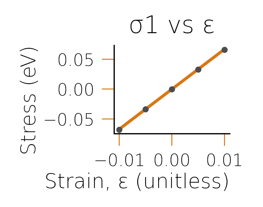
Stress-strain curve for \(\sigma_1\) (corresponding to \(C_{11}\) part).

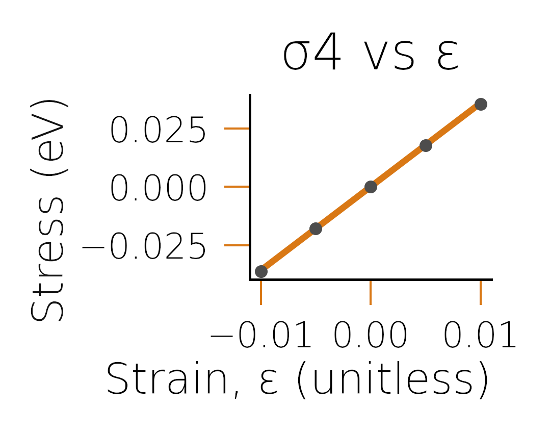
Stress-strain curve for \(\sigma_4\) (corresponding to \(C_{44}\) part).

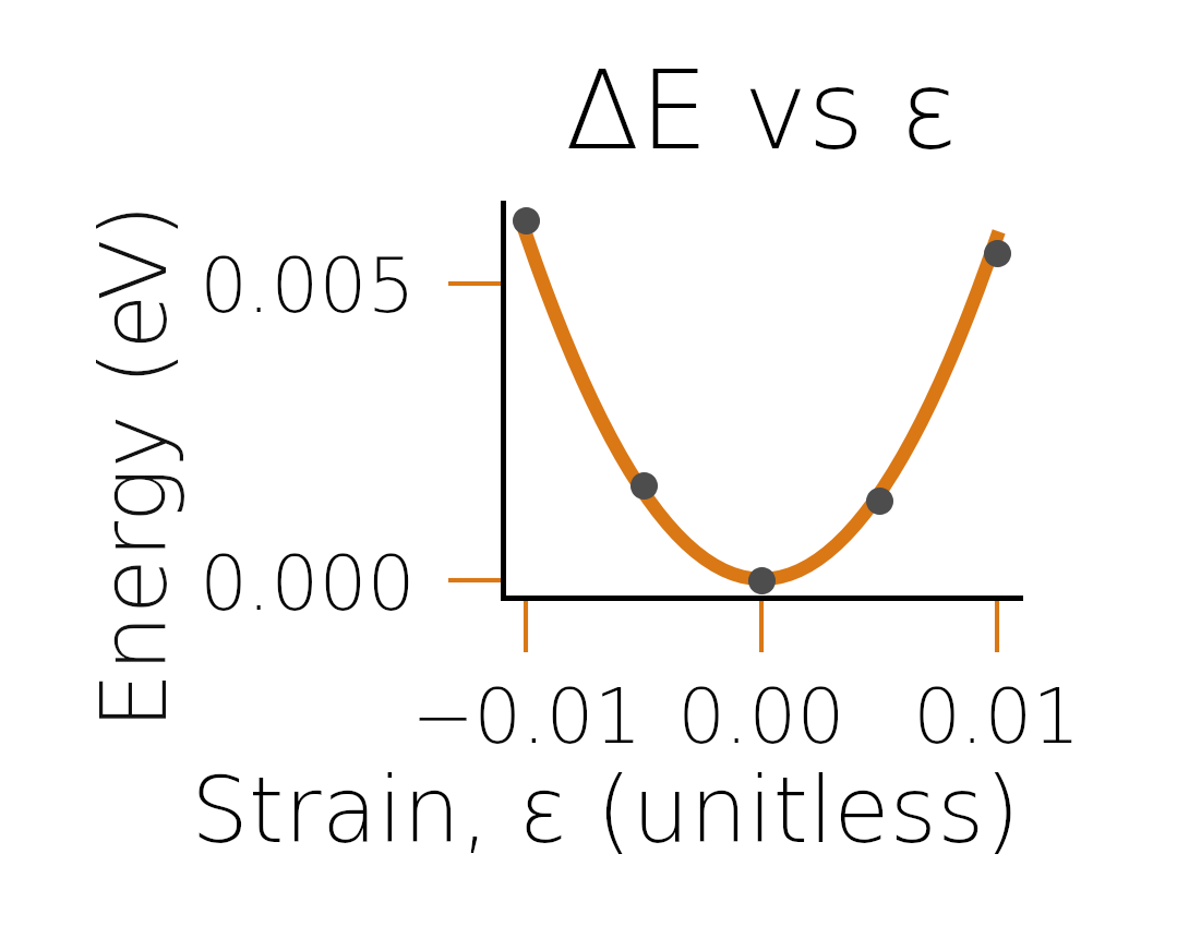
Energy-strain curve for given strain.

[Jamal2014]

Jamal, M., et al. "Elastic constants of cubic crystals." Computational Materials Science 95 (2014): 592-599.

[Jamal2018]

Jamal, M., et al. "IRelast package." Journal of Alloys and Compounds 735 (2018): 569-579.

[OHESS2020]

Liu, Zhong-Li. “High-efficiency calculation of elastic constants enhanced by the optimized strain-matrix sets." arXiv preprint: arXiv:2002.00005 (2020).

[ULICS]

Yu, R., et al. "Calculations of single-crystal elastic constants made simple." Comput. Phys. Commun. 181 (2010): 671-675.